Implementing an Artificial Neural Network from Scratch in Python

Introduction

This tutorial will walk you through how to implement a densely connected artificial neural network from scratch in Python. Throughout this tutorial, we’re going to build on the concepts we explained in our tutorial on implementing logistic regression from scratch in Python.

Logistic regression is an excellent tool for learning linear boundaries. It can learn to classify linearly separable datasets, which are those in which a straight line between the datasets can separate. If you stack multiple logistic regression units together, you can learn complex decision boundaries and classify non-linearly separable datasets.

The model you get after stacking multiple logistic regression units is called an artificial neural network. These artificial neural networks can learn much more than binary classification. You can perform multi-class classification, multi-label classification, regression and more.

In this tutorial, we’re going to keep things simple by developing a neural network for binary classification. Let’s get to it!

Creating Dummy Dataset

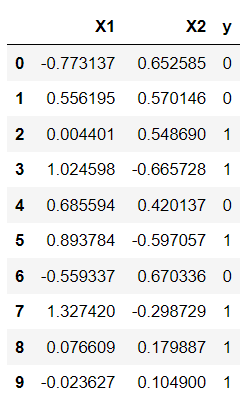
The following script creates a non-linearly separable dataset with 1000 samples and two features.

from sklearn.datasets import make_blobs, make_moons

X, y = make_moons(n_samples=1000, noise = 0.1)

import pandas as pd

dataset = pd.DataFrame(X, columns = ["X1", "X2"])
dataset["y"] = y
dataset.head(10)

Output:

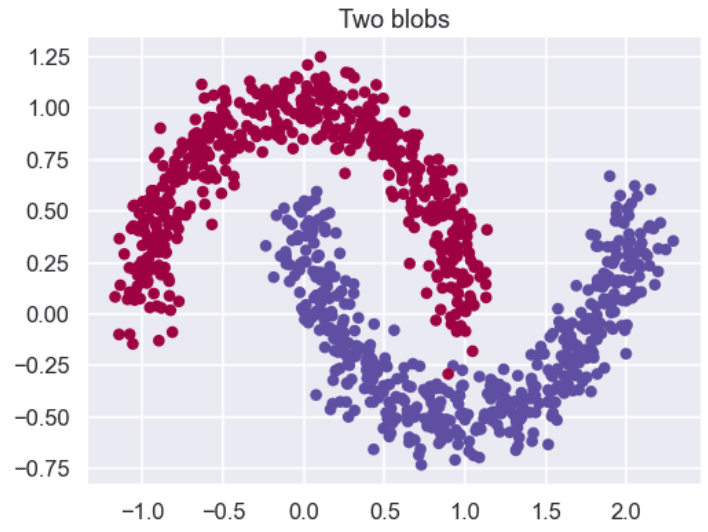
The script below plots our dataset. You can see that the dataset contains two moon-like structures that cradle into one another. You cannot separate this dataset with a straight line.

from matplotlib import pyplot
import seaborn as sns
sns.set_style("darkgrid")
sns.set_context("talk")

pyplot.figure(figsize=(8, 6))
pyplot.title("Two blobs")
pyplot.scatter(X[:, 0], X[:, 1], marker="o", c=y, s=50, cmap ="Spectral")

Output:

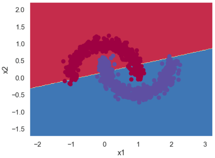
If you use the logistic regression model to classify the above dataset, you will get a decision boundary similar to the one in the following figure. You can see that the model consists of a straight line, and it cannot correctly classify all the points. We’ll show you how to plot decision boundaries, like the one below, a bit later in this tutorial. This image is only for demonstration, at this point.

Let’s see if a neural network can learn this complex boundary.

The following script converts our labels into a column vector.

y = y.reshape(y.shape[0],1)

print(X.shape)
print(y.shape)

Output:

(1000, 2)
(1000, 1)

Finally, the script below divides the dataset into training and test sets. We will train our neural network model on the training set and will evaluate the model on the unseen test set.

from sklearn.model_selection import train_test_split
X_train, X_test, y_train, y_test = train_test_split(X, y, test_size=0.2, random_state=25)

Get Our Python Developer Kit for Free

I put together a Python Developer Kit with over 100 pre-built Python scripts covering data structures, Pandas, NumPy, Seaborn, machine learning, file processing, web scraping and a whole lot more - and I want you to have it for free. Enter your email address below and I'll send a copy your way.

Model Architecture & Weights Initialization

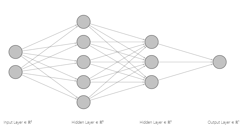
The following figure shows the neural network architecture you’ll implement in this article. It has one input layer with two nodes, two hidden layers with 5 and 3 nodes, and one output layer. The number of nodes in the input and output layers depends on your input features and target labels. Since we have two input features, the input layer consists of two nodes. Likewise, the number of nodes in the output layer corresponds to the single output label.

The choice for the number of layers in the hidden layer of a neural network depends on the decision boundary you want to learn. Adding more nodes and layers enables a neural network to learn more complex decision boundaries.

The number of weights and biases and the shape of each weight depends on your neural network architecture.

From our neural network architecture, you can see that we need three sets of weights and, likewise, three sets of biases.

We use the following naming conventions for our weights matrices:

1. W1: connects the input layer with the first hidden layer. It has shape (2, 5) since there are two nodes in the input layer and five in the first hidden layer.
2. W2: connects the first hidden layer to the second hidden layer and has shape (5, 3).
3. W3: which connects the second hidden layer to the output layer and has the shape (3,1).

Similarly, we define b1, b2, and b3 as the bias values for the corresponding weights.

The following script initializes the weights and biases and prints their shapes and values in the output:

import numpy as np

input_features = X.shape[1]
hidden_layer1_nodes = 5
hidden_layer2_nodes = 3
output_nodes = 1

W1 = np.random.rand(X.shape[1], hidden_layer1_nodes)
b1 = np.zeros((1, hidden_layer1_nodes))

W2 = np.random.rand(hidden_layer1_nodes, hidden_layer2_nodes)
b2 = np.zeros((1, hidden_layer2_nodes))

W3 = np.random.rand(hidden_layer2_nodes, output_nodes)
b3 = np.zeros((1,output_nodes))

print("=== Hidden layer 1 weights and bias ===")
print(W1.shape)
print(W1)
print(b1.shape)
print(b1)

print("=== Hidden layer 2 weights and bias ===")
print(W2.shape)
print(W2)
print(b2.shape)
print(b2)


print("=== Output layer weights and bias ===")
print(W3.shape)
print(W3)
print(b3.shape)
print(b3)

Output:

=== Hidden layer 1 weights and bias ===
(2, 5)
[[0.25507285 0.49200558 0.18033117 0.8076391  0.94832727]
 [0.3672366  0.07862445 0.11087905 0.1499215  0.22173011]]
(1, 5)
[[0. 0. 0. 0. 0.]]
=== Hidden layer 2 weights and bias ===
(5, 3)
[[0.9568752  0.12273496 0.04722568]
 [0.41575515 0.39888438 0.27229583]
 [0.43131297 0.09711146 0.31365061]
 [0.06710198 0.07220234 0.31065423]
 [0.11245667 0.02636645 0.00889949]]
(1, 3)
[[0. 0. 0.]]
=== Output layer weights and bias ===
(3, 1)
[[0.39603838]
 [0.58832471]
 [0.51062766]]
(1, 1)
[[0.]]

Forward Pass

The forward pass calculates the output of the neural network given some input.

This is going to sound mathematically intense, so bear with us. The forward pass is going to perform the following steps:

1. Take the dot product of input features X weights matrix W1 and add the bias b. The result is assigned to the variable Z1. We then perform the tanh activation function on Z1 to get the activation A1 of the first hidden layer.
2. Take the dot product of the first hidden layer activation A1 with the weights matrix W2 and add the bias b2. Apply the activation tanh on the result Z1 to get the second layer activation A2.
3. Finally, take the dot product of the second hidden layer activation A2 with the weights matrix W3 and add the bias b2. Apply the activation sigmoid function on the result Z2 to get the output layer activation A3.

Notice we apply the sigmoid activation on the output layer and tanh activation on the hidden layers. The sigmoid activation function performs binary classification. For the hidden layer activations, you can use other activation functions such as relu, or leaky relu.

def sigmoid(x):
    s = 1/(1+np.exp(-x))
    return s

The script below defines the make_predictions() function that performs the forward pass.

def make_predictions(X, W1, W2, W3, b1, b2, b3):
    Z1 = np.dot(X,W1) + b1
    A1 = np.tanh (Z1)   # dimensions = (100, 4)

    Z2 = np.dot(A1,W2) + b2
    A2 = np.tanh (Z2)

    Z3 = np.dot(A2,W3) + b3
    A3 = sigmoid (Z3)

    return A1, A2, A3

As we did in our [tutorial on logistic regression]/python/logistic-regression-from-scratch-in-python/), we’re going to calculate the loss using the binary cross-entropy function.

def calculate_loss(Y,Y_hat):

    loss = - np.mean(((Y * np.log(Y_hat)) + ((1-Y)*np.log(1-Y_hat))))

    return loss

Let’s make predictions using the randomly initialized weights values.

A1, A2, predictions = make_predictions(X_test, W1, W2, W3, b1, b2, b3)

y_pred = [1 if pred > 0.5 else 0 for pred in predictions]

from sklearn.metrics import classification_report
from sklearn.metrics import accuracy_score

print(classification_report(y_test, y_pred))
print(accuracy_score(y_test, y_pred))

Output:

precision    recall  f1-score   support

0       0.67      0.18      0.28       100
1       0.53      0.91      0.67       100

accuracy                           0.55       200
macro avg       0.60      0.55      0.48       200
weighted avg       0.60      0.55      0.48       200

0.545

The output shows that we get an accuracy of 54.5% using the randomly initialized weights. Like logistic regression, the central idea in neural networks is to find weights that minimize the loss function. Minimizing the loss function results in the best possible predictions.

One way to minimize the loss function is to take partial derivatives of the loss function with respect to all the weights and biases in a neural network. The partial derivative tells us if the loss value increases or decreases against the current weight value. A fraction of the derivative (fraction specified by the learning rate) is then subtracted from the current weight values. This process is called gradient descent.

The following two scripts implement the gradient descent algorithm for the binary cross-entropy loss function. Here’s a good article if you want to dive into the mathematical details of the gradient descent for binary cross entropy loss function.

The find_gradient() method finds the partial derivates of weights and biases with respect to the binary cross entropy loss function.

Get Our Python Developer Kit for Free

I put together a Python Developer Kit with over 100 pre-built Python scripts covering data structures, Pandas, NumPy, Seaborn, machine learning, file processing, web scraping and a whole lot more - and I want you to have it for free. Enter your email address below and I'll send a copy your way.

Backpropagation

def find_gradient(X, Y, W1, b1, W2, b2, W3, b3, A1, A2, A3):

    dZ3 = A3-Y
    dw3 = np.dot(A2.T, dZ3)/X.shape[0]
    db3 = (np.sum(dZ3,axis=0, keepdims=True))/X.shape[0]

    dZ2 = np.dot(dZ3, W3.T) * (1 - np.power(A2,2))
    dw2 = np.dot(A1.T, dZ2)/X.shape[0]
    db2 = (np.sum(dZ2, axis=0, keepdims=True))/X.shape[0]

    dZ1 = np.dot(dZ2, W2.T) * (1 - np.power(A1,2))
    dw1 = np.dot(X.T, dZ1)/X.shape[0]
    db1 = (np.sum(dZ1, axis=0, keepdims=True))/X.shape[0]


    return dw1, db1, dw2, db2, dw3, db3

The update_weights() method in the script below updates the weight values by subtracting weight gradients from the current weight values.

def update_weights(W1, b1, W2, b2, W3, b3, dw1, db1, dw2, db2, dw3, db3):
    W1 = W1 - lr * dw1
    b1 = b1 - lr * db1

    W2 = W2 - lr * dw2
    b2 = b2 - lr * db2

    W3 = W3 - lr * dw3
    b3 = b3 - lr * db3

    return W1, b1, W2, b2, W3, b3

Training the Neural Network Model

The script below defines the train_model() method that trains our neural network for a specific number of features (defined by epochs).

def train_model(X, y, W1, b1, W2, b2, W3, b3, epochs, lr):  

    lr = lr

    loss_vals = []

    for i in range(epochs):

        ## Forward Pass
        A1, A2, A3 = make_predictions(X, W1, W2, W3, b1, b2, b3)
        loss = calculate_loss(y, A3)

        if (i%100) == 0:
            print("loss at iteration" , i, loss)
        loss_vals.append(loss)

        ## Back Propagation
        dw1, db1, dw2, db2, dw3, db3 = find_gradient(X, y, W1, b1, W2, b2, W3, b3, A1, A2, A3)

        W1, b1, W2, b2, W3, b3 = update_weights(W1, b1, W2, b2, W3, b3, dw1, db1, dw2, db2, dw3, db3)

    return W1, b1, W2, b2, W3, b3, loss_vals

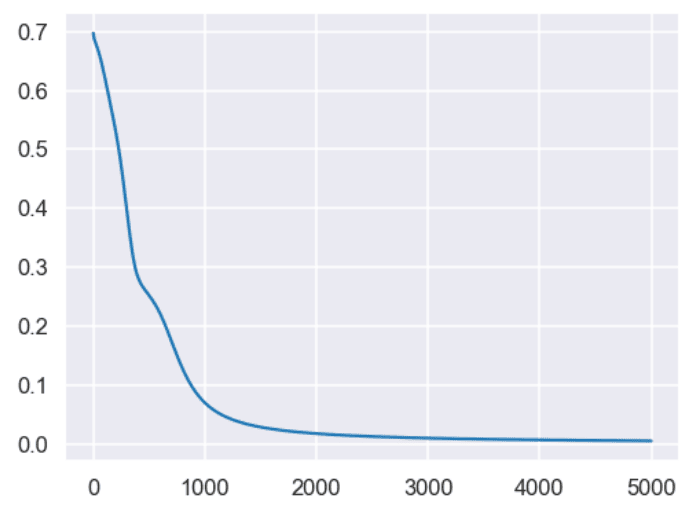
Let’s train our model on the dataset for 5 thousand epochs. The loss is printed after every 100 epochs. The output displays the last ten loss values.

lr = 0.1
epochs = 5000

W1, b1, W2, b2, W3, b3, loss_vals = train_model(X_train, y_train, W1, b1, W2, b2, W3, b3, epochs, lr)

Output:

loss at iteration 4000 0.006519962197880361
loss at iteration 4100 0.006312642729394372
loss at iteration 4200 0.006116876604983178
loss at iteration 4300 0.005931705130904944
loss at iteration 4400 0.005756275298527049
loss at iteration 4500 0.005589825548080949
loss at iteration 4600 0.005431673755483966
loss at iteration 4700 0.00528120705175335
loss at iteration 4800 0.005137873160318173
loss at iteration 4900 0.0050011729972679305

The script below plots the loss values against the number of epochs. In the output, you can see that our loss decreases rapidly up to 1000 epochs and decreases very slowly for the subsequent 4000 iterations.

pyplot.figure(figsize=(8, 6))

x = [loss_vals.index(i) for i in loss_vals]
pyplot.plot(x, loss_vals)
pyplot.show()

Output:

Making Predictions and Evaluating the Model

Our model is trained. Let’s make predictions on our test set using the updated weights and biases values.

from sklearn.metrics import classification_report
from sklearn.metrics import accuracy_score

A1, A2, predictions = make_predictions(X_test, W1, W2, W3, b1, b2, b3)
y_pred = [1 if pred > 0.5 else 0 for pred in predictions]

print(classification_report(y_test, y_pred))
print(accuracy_score(y_test, y_pred))

Output:

The output shows that we get 100% accuracy on the test set.

precision    recall  f1-score   support

0       1.00      1.00      1.00       105
1       1.00      1.00      1.00        95

accuracy                           1.00       200
macro avg       1.00      1.00      1.00       200
weighted avg       1.00      1.00      1.00       200

1.0

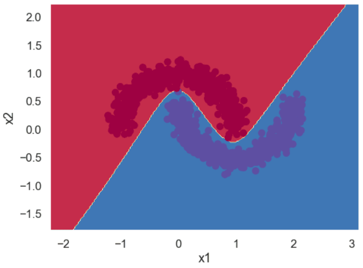
Finally, you can plot a decision boundary for your trained neural network using the following script. The output shows that our model has successfully learned the non-linear decision boundary that separates the two classes in our label set.

import matplotlib.pyplot as plt
sns.set_style("darkgrid")
sns.set_context("talk")

def plot_decision_boundary(model, X, y):

    # find the minimum and maximum values for the first
    # and second feature of the dataset

    x_min, x_max = X[:, 0].min() - 1, X[:,0].max() + 1
    y_min, y_max = X[:, 1].min() - 1, X[:, 1].max() + 1
    h = 0.02

    # generate a grid of data points between maximum and minimum feature values
    xx, yy = np.meshgrid(np.arange(x_min, x_max, h), np.arange(y_min, y_max, h))

    # make prediction on all points in the grid
    A1, A2, Z = model(np.c_[xx.ravel(), yy.ravel()])
    Z = Z.reshape(xx.shape)

    # convert sigmoid outputs to binary
    Z = np.where(Z > 0.5, 1, 0)

    # plot countourf plot to fill the grid with data points
    # the colour of the data points correspond to prediction (0 or 1)
    plt.contourf(xx, yy, Z, cmap=plt.cm.Spectral)

    # plot the original scatter plot to see where the data points fall
    plt.ylabel('x2')
    plt.xlabel('x1')
    plt.scatter(X[:, 0], X[:, 1], c=y, cmap=plt.cm.Spectral)

plt.figure(figsize=(8, 6))
plot_decision_boundary(lambda x: make_predictions(x, W1, W2, W3, b1, b2, b3), X, y)

Output:

This is just the tip of the iceberg; neural networks can learn far more complex boundaries, as you will see in our upcoming tutorials. Subscribe below to get notified when we publish them!

Get Our Python Developer Kit for Free

I put together a Python Developer Kit with over 100 pre-built Python scripts covering data structures, Pandas, NumPy, Seaborn, machine learning, file processing, web scraping and a whole lot more - and I want you to have it for free. Enter your email address below and I'll send a copy your way.