Using Python TensorFlow 2.0 for Regression Tasks

Our last tutorial described how to use TensorFlow for Data Classification. In this article, we’ll teach you how to perform regression tasks with Python’s TensorFlow 2.0. You’ll develop a simple deep learning model capable of predicting the price of Diamonds. This is going to be a fun tutorial, so let’s get started!

Environment Setup

Before you can create a deep learning model for regression in TensorFlow 2.0, you have to install and import a few libraries.

To install the TensorFlow 2.0 library, you can use pip installer. The following command installs the TensorFlow 2.0 library:

$ pip install tensorflow

If you have an old version of TensorFlow already installed, you can update your TensorFlow to version 2.0 via the following command:

pip install --upgrade tensorflow

The other libraries you will need to install in order to execute the scripts in this tutorial are Pandas, Seaborn, NumPy, Scikit-Learn, and Matplotlib. The following script installs these libraries:

pip install matplotlib
pip install seaborn
pip install pandas
pip install NumPy
pip install scikit-learn

Import Required Libraries

Before we actually perform regression with TensorFlow 2.0, let’s first import the seaborn, matplotlib, pandas and TensorFlow modules that we’re going to need in this tutorial:

import seaborn as sns
import pandas as pd
import numpy as np

from tensorflow.keras.layers import Input, Dense, Dropout, Activation
from tensorflow.keras.models import Model

You’re going to see how we use each of these libraries a little later in this tutorials.

You can check the version of the TensorFlow installed on your system by executing the following Python Script:

tf.__version__

As of the date of this publication, you should see “2.0.0” in the output.

Importing and Preprocessing the Dataset

We’ll be performing regression on the diamonds dataset. You don’t need to download the diamonds dataset since it comes prebuilt with the Seaborn library. Execute the following script to import and display the first five rows of the dataset:

reg_dataset = sns.load_dataset('diamonds')
reg_dataset.head()

Output:

The output shows that the dataset has 10 columns. We’ll be predicting the values in the price column based on the values in all the remaining columns.

Let’s see the shape of our dataset.

reg_dataset.shape

Output:

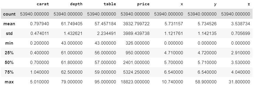
(53940, 10)

The output shows that our dataset contains 53940 rows and 10 columns. To display the statistical information about the numeric columns, you can use the describe() method as shown below.

reg_dataset.describe()

Output:

Get Our Python Developer Kit for Free

I put together a Python Developer Kit with over 100 pre-built Python scripts covering data structures, Pandas, NumPy, Seaborn, machine learning, file processing, web scraping and a whole lot more - and I want you to have it for free. Enter your email address below and I'll send a copy your way.

One Hot Encoding of Categorical Columns

If you look at the dataset, you can see that we have some columns with categorical or string type values e.g. cut, color, and clarity. Deep learning models in TensorFlow requires the training data be in numeric format. Therefore, we need to convert these categorical values to numeric values. One of the ways to convert categorical values to numeric is via one hot encoding. Here are the steps to perform one hot encoding of a categorical column:

Step 1: For each unique value in the original categorical column, you create a new column. In our example, the cut column contains five unique values, as demonstrated here:

list(reg_dataset.cut.unique())

Output:

['Ideal', 'Premium', 'Good', 'Very Good', 'Fair']

To one hot encode the cut column, you’ll need to create 5 columns. Technically, you only need 4 columns since if the cut isn’t one of the first 4 types, it must be the 5th type. We’ll demonstrate this in Step 2.

Step 2: Next, among the new columns, add one to the column that corresponds to the original value in the cut For instance, in the first record, the value for the cut column is Ideal. You will add 1 in the newly created Ideal column. All the newly created remaining columns for cut column will have values of zeros if the cut doesn’t match Ideal.

This will be more clear with an example. Let’s first remove the cut, color, and clarity columns from our dataset and one hot encode them.

numeric_data= reg_dataset.drop(['cut','color', 'clarity'], axis=1)

To one hot encode a column, you can use the pd.get_dummies() method as shown below.

cut_onehot = pd.get_dummies(reg_dataset.cut).iloc[:,1:]
color_onehot = pd.get_dummies(reg_dataset.color).iloc[:,1:]
clarity_onehot = pd.get_dummies(reg_dataset.clarity).iloc[:,1:]

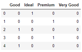
Let’s now print the one hot encoded columns for the original cut column.

cut_onehot.head()

Output:

From the output, you can see that 4 columns have been created instead of 5. A column for value fair has not been created. This is because a categorical column with N unique values can be one hot encoded via N-1 columns. For instance, if there is a 0 in all the above four columns, that will implicitly mean that this record has the cut value of fair.

Step 3: Next, we need to concatenate the one hot encoded columns we just created with the numeric columns in the original dataset.

reg_dataset = pd.concat([numeric_data,cut_onehot, color_onehot,clarity_onehot], axis=1)
reg_dataset.head()

Here is how our final dataset looks.

Output:

Dividing the Data into Training and Test Sets

Before we can train our deep learning models, we need to divide the data into feature and label sets. Our feature set will consist of all the columns except the price column whereas the label set will consist of the values solely from the price column.

features = reg_dataset.drop(['price'], axis=1).values

labels = reg_dataset['price'].values

Notice we use the drop command to quickly exclude a column from our features set.

In machine learning and deep learning, data is divided into the training and test sets. The training set is used to train a deep learning model while the test set is used to evaluate the performance of the trained model. The following script divides the data into an 80% training set and a 20% test set. This ratio is defined by the test_size attribute of the train_test_split() function as shown below:

from sklearn.model_selection import train_test_split

X_train, X_test, y_train, y_test = train_test_split(features, labels, test_size=0.2, random_state=40)

Next, before we train our deep learning model, we need to scale our data. Scaling can be useful since the magnitude of data in different columns can vary greatly. It’s a good practice to scale the dataset so that all the columns have similar data scales.

from sklearn.preprocessing import StandardScaler

sc = StandardScaler()
X_train = sc.fit_transform(X_train)
X_test = sc.transform(X_test)

Training Regression Models in TensorFlow 2.0

Defining TensorFlow models

In this example, our TensorFlow model will be simple. It will consist of a densely connected neural network. If you are not familiar to neural networks, check out this link.

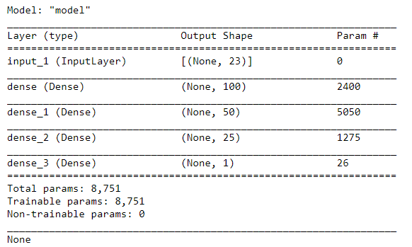
Our neural network will contain an input layer, three hidden layers and one output layer. The hidden layers will be densely connected. The first layer contains 100 neurons, the second hidden layer contains 50 neurons, and the third hidden layer contains 25 neurons. You can play around with these values to see if you get better results. Since the output is a single value, i.e. the price of diamond, the output layer will contain only 1 neuron. The following script defines our model.

input_layer = Input(shape=(features.shape[1],))
l1 = Dense(100, activation='relu')(input_layer)
l2 = Dense(50, activation='relu')(l1)
l3 = Dense(25, activation='relu')(l2)
output = Dense(1)(l3)

The above script creates our neural network model. To compile the model, the compile() method is used. To connect previous layer to the next layer, you simply add the previous layer name inside the parenthesis that follow the next layer name.

Next you need to compile the model. To compile the model, the compile() method is used.

model = Model(inputs=input_layer, outputs=output)
model.compile(loss="mean_absolute_error" , optimizer="adam", metrics=["mean_absolute_error"])

Let’s print the model summar. To do so, you can use the summary() method of the model object.

print(model.summary())

Output:

Once the model is created, you have can train it by simply calling the fit() method. The method requires you pass it the training set (i.e. the training features and labels, the batch size and the number of epochs). The batch size refers to the number of records processed at once and the epochs argument refers to the number of iterations for which the model will be trained on the complete dataset. Here’s how you call the .fit() method:

history = model.fit(X_train, y_train, batch_size=2, epochs=20, verbose=1, validation_split=0.2)

While the model is being trained, you can see the accuracy obtained after each epoch. The output below only shows the results from the last 5 epochs, but you should see result from all 20 epochs.

Output:

2.0520 - val_mean_absolute_error: 352.0527
Epoch 17/20
34521/34521 [==============================] - 28s 820us/sample - loss: 320.8634 - mean_absolute_error: 320.8634 - val_loss: 372.6321 - val_mean_absolute_error: 372.6329
Epoch 18/20
34521/34521 [==============================] - 28s 825us/sample - loss: 320.5240 - mean_absolute_error: 320.5243 - val_loss: 361.3044 - val_mean_absolute_error: 361.3043
Epoch 19/20
34521/34521 [==============================] - 29s 849us/sample - loss: 318.1330 - mean_absolute_error: 318.1321 - val_loss: 364.1879 - val_mean_absolute_error: 364.1886
Epoch 20/20
34521/34521 [==============================] - 37s 1ms/sample - loss: 316.9341 - mean_absolute_error: 316.9344 - val_loss: 353.8328 - val_mean_absolute_error: 353.8323

Evaluating Model performance

Now that our diamond price model is trained with TensorFlow 2.0, we can see how good our regression model is. To evaluate the performance of a regression, the most commonly used metric is the mean absolute error, which gives us the average error between the predicted and actual values across all the test examples. The following script finds the mean absolute error for our training and testing set.

from sklearn.metrics import mean_absolute_error
from math import sqrt

pred_train = model.predict(X_train)
print(mean_absolute_error(y_train,pred_train))

pred = model.predict(X_test)
print(mean_absolute_error(y_test,pred))

Output:

319.3074745419382

324.4026458055654

The output shows that on average, there is a difference of only $324 between the predicted and actual values and the values predicted by our model. This is less than 10% of the average values of all the diamonds in our dataset ($3932.79) which means our model is pretty accurate.

Complete Code

To help you build your own regression model, here’s our complete code for predicting diamond prices using Tensorflow 2.0 in this tutorial:

import seaborn as sns
import pandas as pd
import numpy as np
import tensorflow as tf

from tensorflow.keras.layers import Input, Dense, Dropout, Activation
from tensorflow.keras.models import Model

tf.__version__

reg_dataset = sns.load_dataset('diamonds')
reg_dataset.head()

reg_dataset.shape

reg_dataset.describe()

list(reg_dataset.cut.unique())

numeric_data= reg_dataset.drop(['cut','color', 'clarity'], axis=1)

cut_onehot = pd.get_dummies(reg_dataset.cut).iloc[:,1:]
color_onehot = pd.get_dummies(reg_dataset.color).iloc[:,1:]
clarity_onehot = pd.get_dummies(reg_dataset.clarity).iloc[:,1:]

cut_onehot.head()

reg_dataset = pd.concat([numeric_data,cut_onehot, color_onehot,clarity_onehot], axis=1)

reg_dataset.head()

features = reg_dataset.drop(['price'], axis=1).values

labels = reg_dataset['price'].values

from sklearn.model_selection import train_test_split

X_train, X_test, y_train, y_test = train_test_split(features, labels, test_size=0.2, random_state=40)

from sklearn.preprocessing import StandardScaler

sc = StandardScaler()
X_train = sc.fit_transform(X_train)
X_test = sc.transform(X_test)

input_layer = Input(shape=(features.shape[1],))
l1 = Dense(100, activation='relu')(input_layer)
l2 = Dense(50, activation='relu')(l1)
l3 = Dense(25, activation='relu')(l2)
output = Dense(1)(l3)

model = Model(inputs=input_layer, outputs=output)
model.compile(loss="mean_absolute_error" , optimizer="adam", metrics=["mean_absolute_error"])

print(model.summary())

history = model.fit(X_train, y_train, batch_size=2, epochs=20, verbose=1, validation_split=0.2)

from sklearn.metrics import mean_absolute_error
from math import sqrt

pred_train = model.predict(X_train)
print(mean_absolute_error(y_train,pred_train))

pred = model.predict(X_test)
print(mean_absolute_error(y_test,pred))

For more Python programs like this, subscribe using the form below:

Get Our Python Developer Kit for Free

I put together a Python Developer Kit with over 100 pre-built Python scripts covering data structures, Pandas, NumPy, Seaborn, machine learning, file processing, web scraping and a whole lot more - and I want you to have it for free. Enter your email address below and I'll send a copy your way.