The Data Revolution is upon us, and everyone wants to gather and analyze as much data as possible. Spreadsheets like Excel offer one of the best ways to engage in data analysis for the average worker - that is, those without the need for distributed systems or supercomputers. Within spreadsheets, one of the most powerful tools for analyzing data and extracting information is a Pivot Table. In this tutorial, we’ll automate pivot tables using VBA so you can easily set up new ones or hand off your files to a coworker.
Like my VBA API tutorial, this one may be a little complicated due to the number of functions and concepts involved. However, just like APIs, Pivot Tables are immensely powerful and it is worthwhile to learn the concepts here. Data is the future, and if you can programmatically create Pivot Tables to analyze that data, you are ahead of the curve.
Your Data Source
First, you’ll need a data source. If you already have the data in your spreadsheet, great. If not, you can find plenty of open data sources online. Most governments and international bodies collect and publish massive amounts of data, and many companies also produce open data sets.
For this tutorial, I will use the Air Quality Index for all United States CBSAs (Census Bureau Statistical Areas). This is the air quality for every city/town in the country, and it is accessible on the EPA’s website here.
The following attributes, among others, are included in the dataset:
- CBSA (town or city area)
- AQI (air quality index)
- Category (descriptive term of quality, such as “good” or “hazardous”)
- Particulate type (PM2.5, PM5, PM10, SO2, etc.)
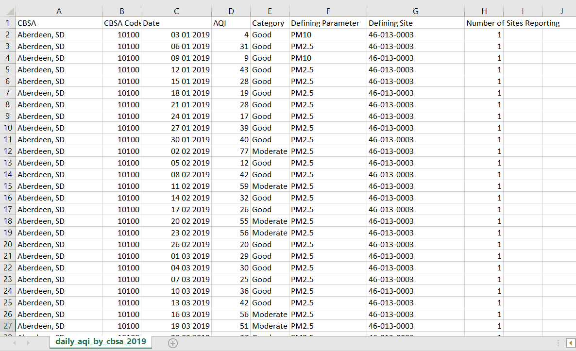
The particular set I retrieved had about 110,000 instances, so there is quite a lot of data here - perfect for Pivot Table analysis. From the snapshot below you can see that it populates Columns A to H:

2019 Dataset from the EPA for Air Quality Index (AQI)
Creating the Pivot Table
You’ll probably want to preserve the original data, so it’s best to put your Pivot Table on a new sheet, which can easily be accomplished with the Sheets.Add function in VBA. This function adds a new Sheet object to the Sheets collection of your workbook
Select the Data
First, grab the data you want to manipulate in the table. Since our data populates Columns A through H, you can identify and set a Range object with a simple column selection:
Set ODRange = Range("A:H")If you use another dataset, you will need to find the bounds independently - this can be done programmatically. There are several ways to do this, but it’s important to capture the entire column since the number of rows in your table may change. One common way is to set your Range object equal to the entire used range, like this
Set ODRange = ActiveSheet.UsedRange.EntireColumnCreate the Sheet
I recommend assigning the new sheet to a named Object. This line creates the new Sheet object, which you can later reference (in the same macro) by calling
Set PTSheet = Sheets.Add
PTSheet.Name = "Pivot Sheet"
Cache the Data
VBA requires you to cache the data before supplying it to the Pivot Table creation function. This ensures Excel knows where to find the source when you want to refresh the table. It basically creates a map in the computer’s memory between the Pivot Table and the Source Data, so changes can easily flow between the two.
To cache, you need to add it to the workbook’s aptly name PivotCaches collection:
Set PTCache = ThisWorkbook.PivotCaches.Create(xlDatabase, ODRange)Create and Place the Table
Now just put the table in the right place and give it a title:
Set PT = PTCache.CreatePivotTable(PTSheet.Cells(1, 1), "AQI for CBSAs 2019")If you visually inspect
Sometimes you can get a run-time error 5, Invalid procedure or argument, when establishing your Pivot Table with VBA. Older version of Excel can be picky and require the SourceData argument in the PivotCaches.Create function to be delivered as an R1C1 style string instead of as a Range argument.
You can also get the run-time 5 error if the optional Version argument of the PivotCaches.Create function doesn’t match the DefaultVersion argument in the CreatePivotTable function. We didn’t declare any of these parameters when we made our PivotTable, but it’s something to keep in mind if you run into trouble.
Make powerful macros with our free VBA Developer Kit It’s easy to copy and paste a macro like this, but it’s harder make one on your own. To help you make macros like this, we built a free VBA Developer Kit and wrote the Big Book of Excel VBA Macros full of hundreds of pre-built macros to help you master file I/O, arrays, strings and more - grab your free copy below.
Adding Fields and Filters
Of course, the point of Pivot Tables is to manipulate data, so we’ll need to populate the table with the correct data. It is a relatively straightforward process if you already know how to manipulate Pivot Tables graphically (i.e., using a mouse in Excel).
Let’s add the
Rows are probably the easiest to understand and add. Simply find the name of the field in our new, blank Pivot Table and assign it the xlRowField orientation:
To add row fields:
PT.PivotFields("CBSA").Orientation = xlRowFieldFilters are just as easy. Find the name of the original field in the data and assign it the xlPageField orientation:
To add filters:
PT.PivotFields("Category").Orientation = xlPageField
PT.PivotFields("Defining Parameter").Orientation = xlPageField
If you want to add columns, follow the same steps, but use xlColumnField as the orientation.
Adding calculated values
For calculated values, there is one extra step. Excel needs to make some calculations, so we will need to supply a function. Use the AddDataField function and feed it the field to operate on. Here, we will average the xlAverage argument.
To add a (calculated) Values field
PT.AddDataField PT.PivotFields("AQI"), "Average AQI for 2019", xlAverageUsing the Data
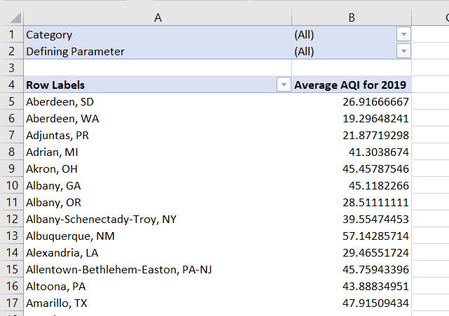
At this point, you should have something like this on

The Pivot Table we just created
Notice there is a problem with the statistical analysis here, though. All numbers for all particulate types are being averaged together. While this can give you some indication of pollution levels, it is probably better to view each particulate individually. You can do this by filtering for each
Switching Orientations
The xlPageField, but we can set it as a column instead to see the breakdown for each city. We’ll need to access the table, find the field, and change it. Remember that we named the table
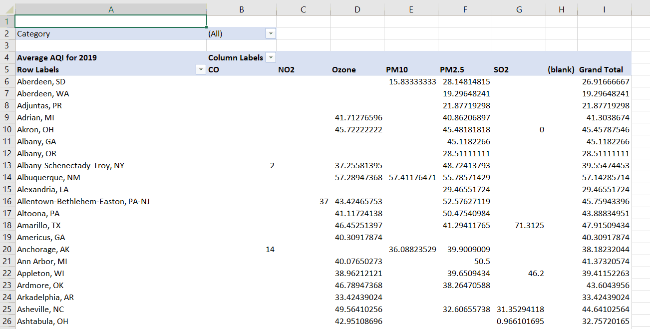
Worksheets("Pivot Sheet").PivotTables("AQI for CBSAs 2019").PivotFields("Defining Parameter").Orientation = xlColumnFieldand now you can see the particulate size average by city along with the average of all particulates:

The new Pivot Table with particulate type broken down
Because the only calculated DataField is the average, switching the orientation of xlSum, we’d have a breakdown by average and by sum.
To recap, we’ve found a data source, created a Pivot Table, added fields and filters, and changed orientations. This was a very basic overview, but it gives you the foundation for setting up Pivot Tables. At this point, you can easily create Pivot Tables in Excel and pass that file to your friends or coworkers. Or you can simplify some of your own tasks when analyzing data. Now go experiment!
Sub create_full_table()

Set ODRange = Range("A:H")
Set PTSheet = Sheets.Add
PTSheet.Name = "Pivot Sheet"
Set PTCache = ThisWorkbook.PivotCaches.Create(xlDatabase, ODRange)
Set PT = PTCache.CreatePivotTable(PTSheet.Cells(1, 1), "AQI for CBSAs 2019")

PT.PivotFields("CBSA").Orientation = xlRowField
PT.PivotFields("Category").Orientation = xlPageField
PT.PivotFields("Defining Parameter").Orientation = xlPageField
PT.AddDataField PT.PivotFields("AQI"), "Average AQI for 2019", xlAverage
Worksheets("Pivot Sheet").PivotTables("AQI for CBSAs 2019").PivotFields("Defining Parameter").Orientation = xlColumnField
End Sub
If you liked this tutorial, we have a 20+ part free email series designed to help you learn more VBA tricks like this one. Check it out using the form below and share this article on Twitter and Facebook.

