The AdvancedFilter method in VBA is a powerful tool we first introduced to get a list of unique values, which is common in applications that deal with large amounts of data. In this tutorial we’ll explore how to use AdvancedFilter to filter on multiple criteria rather than just a single column of data.
The Target Range
We’ll use the same dataset we used in our article for finding unique values. Grab the CSV here or follow along with this screenshot:
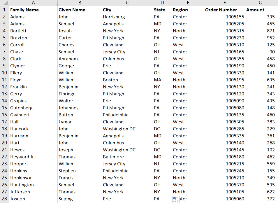
Here we have a list of orders with headers and the associated names, region, US state, and amount.
Targeting the range is as simple as inputting the columns. VBA will treat everything in that column as part of the table. However, if you’d prefer to only filter part of a table, you can explicitly define an ending row when defining your range.
In our case, rows
Range("A:G").AdvancedFilterThe Criteria Range
Rather than take a single criterion, AdvancedFilter considers an entire set of criteria.
So we don’t have to hardcode our criteria in our VBA macro, let’s build a new table with headers matching those in our target range. Then, we’ll add our filtering requirements to this table. Columns
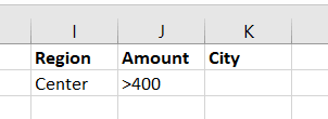
Screenshot of data with just two criteria
You don’t need to cover every header and you don’t have to assign a criteria to each header in the table. Our target Range has 7 fields while our Criteria Range table only has
We can then set our CriteriaRange attribute to the range
Range("A:G").AdvancedFilter CriteriaRange:=Range("I1:J2")We’re still building our AdvancedFilter statement, so the code won’t work just yet. If you try running it now, you’ll get a Run-time error ‘1004’: AdvancedFilter method of Range class failed error because we haven’t defined an Action. This argument tells AdvancedFilter whether to filter in place or copy the filtered results to a new range. We’ll do that later, but I want to step through the code so far.
Make powerful macros with our free VBA Developer Kit It’s easy to copy and paste a macro like this, but it’s harder make one on your own. To help you make macros like this, we built a free VBA Developer Kit and wrote the Big Book of Excel VBA Macros full of hundreds of pre-built macros to help you master file I/O, arrays, strings and more - grab your free copy below.
What we’ve asked AdvancedFilter to do so far is filter all entries in
The range contains the headers/fields and the criteria themselves. Notice that, unlike the Target Range, we don’t enter the whole column. A blank row in the Criteria Range will match all data records, which is not what we want. Conversely, Excel interprets a blank cell (here
Filtering on Multiple Criteria
This is where the power of AdvancedFilter becomes clear. Let’s say we want to analyze all
We can set up the Criteria Range like so:
To set this as the criteria range, we should expand to Column K, like this:
Range("A:G").AdvancedFilter CriteriaRange:=Range("I1:K2")With this single table, we can choose to filter on
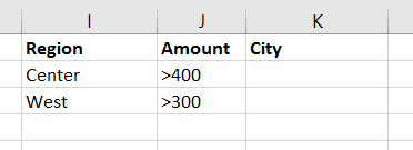
We can also have multiple sets of criteria. We can investigate the Center Region with Amounts greater than $400 OR the West Region with Amounts greater than $300.
To add a second set of criteria, we simply add it to a new row and make sure to expand our Criteria Range in our macro:
Range("A:G").AdvancedFilter CriteriaRange:=Range("I1:K3") 'include Row 3Notice we still don’t have an Action argument defined so this macro still won’t work yet. Don’t worry, we’re getting closer.
AdvancedFilter with AND vs OR
In computing
- AND means all conditions must be met
- OR means at least one condition must be met
With AdvancedFilter criteria ranges, across rows are treated as ANDs while down rows are treated as ORs.
Thus,the previous example was
Center AND >400

OR

West AND >300
AdvancedFilter with Intervals
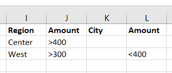
With the mathematical operators (<, >, etc.), you can select intervals, too:
Range("A:G").AdvancedFilter CriteriaRange:=Range("I1:L3")This one will filter for
Center AND >$400

OR

West AND >$300 AND <$400
It’s important to remember ANDs go across rows and ORs go down rows when defining your criteria range tables. If you’re not careful, you could end up with statements like West AND Center AND >$100, which wouldn’t return any records since an order can only be assigned to one
The Output Range
The only mandatory parameter, Action, has two possible values: XlFilterInPlace and XlFilterCopy. You must define one of these XlFilterActions or your AdvancedFilter will fail with a run-time 1004 error.
Using XlFilterInPlace
The XlFilterInPlace action filters the entire Target Range by hiding rows directly in your table. You’ll get all the fields in the output. Let’s use our criteria above for
Center AND >400

OR

West AND >300
We can filter in place with this code using a macro like this:
Sub AdvancedFilterDemo()
Range("A:G").AdvancedFilter Action:=xlFilterInPlace, CriteriaRange:=Range("I1:K3")
End Sub
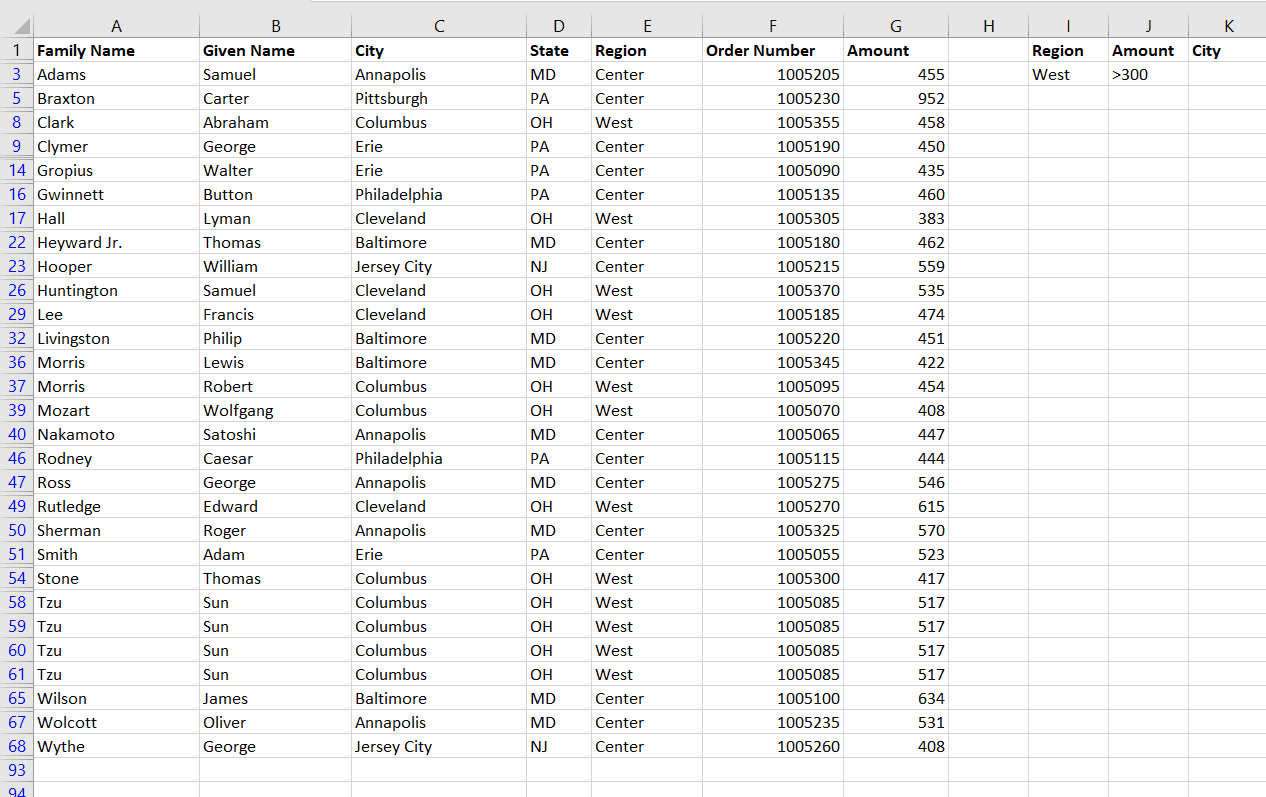
Output FilterInPlace
Unqualifying rows are now hidden, though that does include some of the rows in our Criteria Range table itseflf. This is a very quick way to filter, but it does have the drawback of potentially hiding important rows outside your main table.
Note the duplicate Sun Tzu lines in rows 58 through 61, too. You could use AdvancedFilter to display only one of these by leveraging the Unique parameter.
To unhide all the rows, run this code
ActiveSheet.ShowAllDataOnce you do that, you’ll be back to your original state.
Using XlFilterCopy
In many instances it’s better to copy the output to a new location. This can be another sheet or simply another location on the same sheet.
This method also provides more control over the output, because you can choose which fields to display.
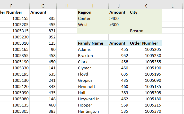
Let’s say you want the criteria
Center AND >400

OR

West AND >300

OR

Boston
but you only want to output
- family name
- amount
- order number
We’ll start the output at Row 6 (light blue) under the same columns as the Criteria Range (light green). You’ll need to manually type out the header names you want in order for the AdvancedFilter macro to know which headers to paste. That’s precisely what we did in light blue, below. Once you type those out, the VBA AdvancedFilter method will know the columns of data you want and it’ll automatically copy the results matching your filter criteria to that location. If you don’t do this, you’ll get a Run-time error ‘1004’: The extract range has a missing or invalid field name error.
Sub AdvancedFilterCopyDemo()
Range("A:G").AdvancedFilter Action:=xlFilterCopy, _
                            CriteriaRange:=Range("I1:K4"), _
                            CopyToRange:=Range("I6:K6")
End Sub
The last parameter, CopyToRange, contains the Range for the headers/fields you select.
The Criteria Range and Output Range don’t really have to share fields at all. For example, we could filter for amounts greater than $500 in the North region and only output the order number. There’s nothing wrong with that. Of course, both ranges must share fields with the original table, otherwise AdvancedFilter won’t know what to do.
Clear Your CopyToRange
If using XlFilterCopy, Excel will guess what to clear in your Output Range. However, you can always be safer by clearing it yourself.
Clear from the first row of data, not from the header row:
Range("I7:K" & Rows.Count).Clear 'headers are in Row 6This method runs very fast and will clear every row of data all the way to the last row of your worksheet.
Taking It Further
By combining XlFilterCopy with multiple sheets, userforms, or even a UsedRange (to identify the bounds of the Criteria Range and Output Range), you can create a very nice tool for your clients or your own data analysis needs.
These steps give a high-level overview for a sophisticated AdvancedFilter tool:
- Place the data table on one sheet
- Put the user-adjustable Criteria Range on another sheet, using Data Validation to restrict headers to those in the table
- Programmatically determine the last row in the Criteria Range sheet uisng End(xlUp).Row or UsedRange.
- Allow users to change output fields under the direction of Data Validation
- Add a button to the criteria page that runs your
AdvancedFiltermacro
Many businesses and organizations leverage Excel for its data manipulation capabilities and AdvancedFilter is one of the quickest ways to get an overview of the data or at least extract the important bits.
You can use the VBA AdvancedFilter method to find matching fields, capture intervals in numerical data and adjust with AND/OR criteria range table structures.
If you found this tutorial useful and you want more tips for writing powerful VBA macros, enter your email address below and I’ll give you my VBA Developer’s Kit for free.

