Timely and effective handling of consumer complaints is essential to customer satisfaction. Companies deploy a substantial number of human resources for consumer complaint handling. However, a part of the process can be automated via modern machine learning models, which can save money and resources.
In this article, we’ll show you how to classify consumer complaints into product categories. To do so, we’ll develop a machine learning model using the Python scikit-learn library. We’re sharing this Python machine learning example as a demonstration to help you when you’re building your own sklearn machine learning model.
Importing the Dataset
Before we import the dataset, let’s import the Python libraries required to run the scripts in this article.
import pandas as pd
import numpy as np
import re

import nltk
nltk.download('stopwords')

from nltk.corpus import stopwords

import matplotlib.pyplot as plt

from sklearn.feature_extraction.text import TfidfTransformer
from sklearn.model_selection import train_test_split

%matplotlib inline
We will use this Consumer Complaints dataset from Kaggle. The dataset contains consumer complaints about various financial products and services.
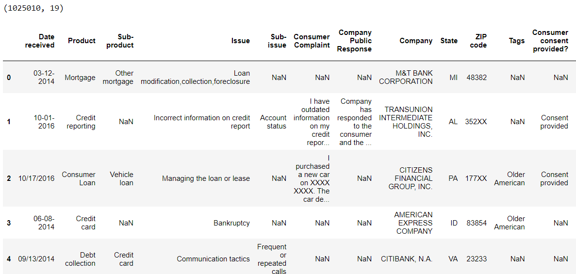
The following script imports the dataset CSV file into a Pandas dataframe. The script prints the dataframe shape and the first five rows.
### Dataset link: https://www.kaggle.com/dushyantv/consumer_complaints

dataset = pd.read_csv(r"C:/Datasets/Consumer_Complaints.csv")
print(dataset.shape)
dataset.head()
Output:
The output shows that the dataset contains more than a million records with 19 columns.
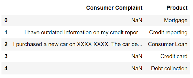
We are only interested in consumer complaints and the corresponding products. Therefore, we filter the
complaints_df = dataset.filter(["Consumer Complaint", "Product"], axis = 1)
complaints_df.head()
Output:
Data Analysis and Preprocessing
A common task when working with large datasets is data cleaning, or preprocessing. We’re going to walk you through what that looks like on this dataset. The following script prints the total number of missing values in our
complaints_df.isnull().sum()Output:
Consumer Complaint    747196
Product                    0
dtype: int64
We’ll remove the records with null values from our dataset. You can remove null values with the Pandas dropna() function as demonstrated in the script below. After dropping the null values, the output confirms that that neither column has null values.
complaints_df.dropna(inplace=True)
print(complaints_df.shape)
complaints_df.isnull().sum()
Output:
(277814, 2)
Consumer Complaint    0
Product               0
dtype: int64
For processing constraints, we’re just going take the first 100k records from our dataset for training and testing the model. You can train your model on more records if you want (and you have the patience to do so).
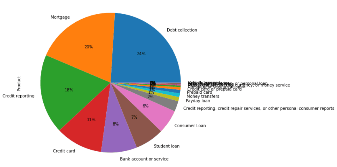
Let’s see a distribution of consumer complaints with respect to product categories from these first 100k records.
complaints_df = complaints_df[:100000]

complaints_df.Product.value_counts().plot(kind='pie',
                                          autopct='%1.0f%%',
                                          figsize=(12, 8))
Output:
The above output shows that the majority of consumer complaints are related to debt collection, followed by mortgage and credit reporting.
The next step is to standardize our text inputs. To do so, we’ll remove all special characters and single characters, then we’ll convert the input text to lowercase. The following script defines and calls the clean_text() function which performs these steps.
def clean_text(text):

    complaints = []

    for comp in text:
        # remove special characters
        comp = re.sub(r'\W', ' ', str(comp))

        # remove single characters
        comp  = re.sub(r'\s+[a-zA-Z]\s+', ' ', comp )

        # Remove single characters from the beginning
        comp  = re.sub(r'\^[a-zA-Z]\s+', ' ', comp)

        # Converting to Lowercase
        comp  = comp.lower()

        complaints.append(comp)

    return complaints

complaints = clean_text(list(complaints_df['Consumer Complaint']))
Finally we need to convert our input text complaints and output product categories into numeric formats. This is necessary since machine learning models work with numbers and not text.
There are numerous strategies for converting text strings to numbers. In this tutorial, we’re going to use the TFIDF approach, which simply takes word presence into account while converting text to numbers.
To implement this approach, use the TfidfVectorizer class from the sklearn.feature_extraction.text module. Here’s an example on how to do this:
from sklearn.feature_extraction.text import TfidfVectorizer
tfid_conv = TfidfVectorizer(max_features=3000, min_df=10, max_df=0.7, stop_words=stopwords.words('english'))
X = tfid_conv.fit_transform(complaints).toarray()
We also need to convert our Product categories into numbers. Here’s one way to do that::
complaints_df['Product'] = complaints_df['Product'].astype('category')
y = list(complaints_df['Product'].cat.codes)
Model Training and Predictions
Now that our model is cleaned up and converted to numeric form, we’re ready to train our sklearn machine learning model on our consumer complaints dataset. The following script divides the inputs and outputs into 80% training and 20% test sets. That means we’re going to train our model using 80% of the data and evaluate its performance on the remaining 20%.
from sklearn.model_selection import train_test_split
X_train, X_test, y_train, y_test = train_test_split(X, y, test_size=0.2, random_state=42)
We’re going to train our text classification model using the Random Forest Classifier, which is the same classifier we used when building our sklearn employee attrition model. If you want to see how the different models impact performance, select one of the other machine learning classifiers from the Scikit-Learn library.
The fit() method of the RandomForestClassifier class from the sklearn.ensemble module can be used to train our model. For making predictions, use the predict() method. This next block trains our machine learning model so it may take a while to run.
from sklearn.ensemble import RandomForestClassifier
classifier = RandomForestClassifier(n_estimators=500, random_state=42)
classifier.fit(X_train, y_train)

y_pred = classifier.predict(X_test)
Now that our model is trained, you can evaluate its performance using classification metrics, like a confusion matrix, accuracy, precision, recall and F1 scores. The following script does that.
from sklearn.metrics import classification_report, confusion_matrix, accuracy_score

print(classification_report(y_test,y_pred))
print(accuracy_score(y_test, y_pred))
Output:
precision    recall  f1-score   support

         0       0.73      0.80      0.76      1646
         1       1.00      0.04      0.07       142
         2       0.75      0.47      0.58       953
         3       0.71      0.78      0.74      2040
         4       0.71      0.02      0.04       233
         5       0.75      0.86      0.80      3428
         6       0.97      0.40      0.56       994
         7       0.79      0.90      0.84      4840
         8       1.00      0.03      0.05        39
         9       0.87      0.21      0.33       164
        10       0.87      0.95      0.91      3732
        11       1.00      0.05      0.10        20
        12       0.85      0.12      0.21       195
        13       1.00      0.02      0.05        43
        14       0.87      0.29      0.44       162
        15       0.87      0.86      0.86      1308
        16       0.00      0.00      0.00        58
        17       0.00      0.00      0.00         3

  accuracy                           0.79     20000
 macro avg       0.76      0.38      0.41     20000
weighted avg       0.80      0.79      0.77     20000

0.79205
The output shows that our model achieves a classification accuracy of 79.2% for consumer complaint classification, which means our model properly classified 79.2% of our test set into the correct product category. That’s not too great. When you see results that aren’t as good as you’d like, you can try increasing the number of training records and you should consider implementing other classification algorithms to see if you can get better performance.


