This tutorial will walk you through how to develop a machine learning employee attrition prediction model with the Python scikit-learn library.
Employee attrition refers to an employees’ voluntary or involuntary departure from an organization. The cost of employee attrition can be huge since replacing human resources with desired skill sets in a limited time is a difficult and costly task.
Knowing in advance the likelihood that employees are going to leave an organization can help organizations make an effort to boost employee retention and proactively hire replacements in time.
Machine learning systems have been developed to flag potential employee attrition, as we’ll demonstrate in this tutorial.
Importing the Dataset
We will use the IBM HR Analytics Employee Attrition Dataset from kaggle to train our machine learning model. If you don’t have a kaggle account, we’ve mirrored the dataset here.
The following script imports the libraries required to run the Python code in this tutorial:
import pandas as pd
import numpy as np
import matplotlib.pyplot as plt
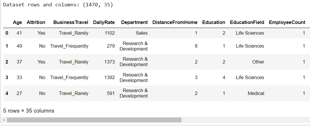
The script below imports the CSV dataset file to a Pandas dataframe. The output shows that we have 1470 rows and 35 columns in our dataset.
attrition_dataset = pd.read_csv(r"C:\Datasets\employee_attrition_dataset.csv")
print("Dataset rows and columns:", attrition_dataset.shape)
attrition_dataset.head()
Output:
Exploratory Data Analysis
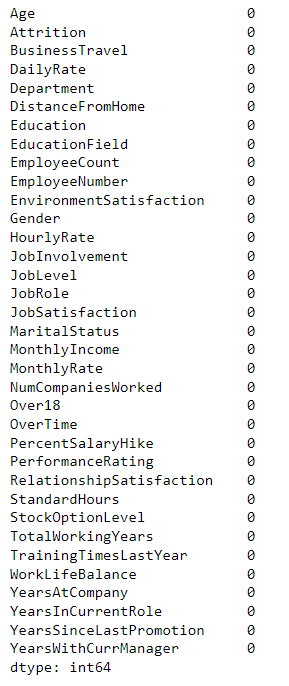
35 columns is quite a bit of data so lets spend a few minutes exploring our dataset. The script below finds the percentage of missing values in each column. The output shows that we don’t have missing values in any column, which is great news!
attrition_dataset.isna().sum()Output:
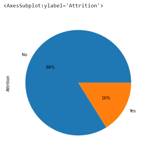
The Attrition column from the dataset contains “Yes” and “No” values for employee attrition. Let’s plot a pie chart showing the data distribution for the “Attrition” column.
attrition_dataset.Attrition.value_counts().plot(kind='pie',
                                                autopct='%1.0f%%',
                                               figsize=(8, 6))
From the output below, you can see that the employee attrition rate in our dataset is 16%, which also means that our dataset is highly imbalanced. We’re not going to employ these techniques here, but we do have a guide describing upsampling and downsampling techniques for handling imbalanced data.
Output:
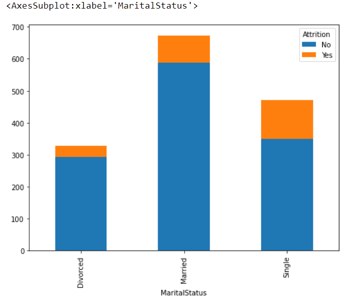
Next, let’s see how the employee attrition ratio varies with the marital status of an employee.
attrition_dataset.groupby(['MaritalStatus', 'Attrition']).size().unstack().plot(kind='bar',
                                                                                stacked=True,
                                                                               figsize=(8, 6))
The output below shows that the attrition rate is the highest among employees with single marital statuses.
Output:
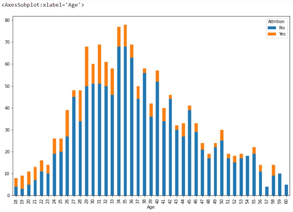
The following script shows the employee attrition rates among different age groups.
attrition_dataset.groupby(['Age', 'Attrition']).size().unstack().plot(kind='bar',
                                                                                stacked=True,
                                                                               figsize=(12, 8))
The output shows that, in our dataset, employee attrition rates are higher among employees aged less than 35. The attrition rates are zero among the employees aged 59 and 60.
Output:
Sometimes it’s valuable to do a little data exploration before diving into what you want to do with your data!
Data Preprocessing
Before you can train a machine learning model on a dataset, you need to do some preprocessing. The first step is to divide the dataset into a features and a labels set. In our dataset the Attrition column contains labels, while the feature set consists of the rest of the columns. The following script divides the dataset into features and labels sets.
feature_set =  attrition_dataset.drop(['Attrition'], axis=1)
labels = attrition_dataset.filter(['Attrition'], axis=1)
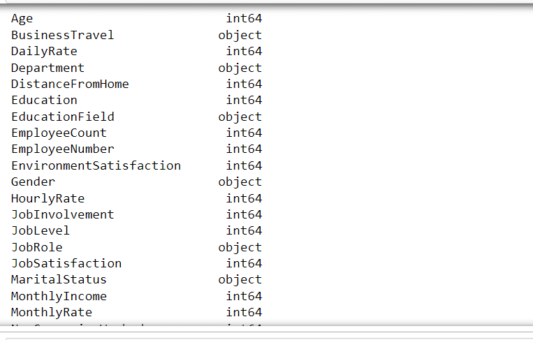
Machine learning algorithms work with numbers, but our feature set contains some non-numeric columns, as you can see from the output of the following script.
feature_set.dtypesOutput:
We need to convert the non-numeric columns in our dataset to numeric columns. Let's do that now.

The following script separates categorical features from numeric features in our dataset.

cat_col_names = ['BusinessTravel',
                       'Department',
                       'EducationField',
                       'Gender',
                       'JobRole',
                       'MaritalStatus',
                       'Over18',
                       'OverTime'
                      ]

num_cols = feature_set.drop(cat_col_names, axis=1)
cat_columns = feature_set.filter(cat_col_names, axis = 1)
You can use the one-hot encoding approach to convert categorical features to numeric features. The following script uses the Pandas get_dummies() method to convert categorical features in our dataset to one-hot encoded numeric features. The output shows the total number of one-hot encoded columns.
cat_columns_one_hot = pd.get_dummies(cat_columns, drop_first=True)
cat_columns_one_hot.shape
Output:
(1470, 21)Finally, you can concatenate the default numeric features with the one-hot encoded numeric features to form the final feature set.
X = pd.concat([num_cols,cat_columns_one_hot], axis=1)
X.shape
Output:
(1470, 47)Similarly, we can convert the simple “Yes” and “No” values from our labels set to binary 1 and 0 values, respectively, using the following script:
y =  labels['Attrition'].map({'Yes': 1, 'No': 0})
y.head()
Output:
0    1
1    0
2    1
3    0
4    0
Name: Attrition, dtype: int64
Alright, our dataset has been cleaned and we’re ready to train our machine learning model.
Model Training and Predictions
We’ll divide our data into training and test sets. The model will be trained using the training set while the performance of the trained model will be evaluated on the test set. The following script divides the data into 80% training and 20% test sets.
from sklearn.model_selection import train_test_split
X_train, X_test, y_train, y_test = train_test_split(X, y, test_size = 0.20, random_state = 42)
Our machine learning model will be trained using the Random Forest Classifier. To do so, we will use the RandomForestClassifier class from the scikit-kearn library. If you want to see how other classifiers perform, feel free to select one of the other machine learning classifiers from the scikit-learn library.
The following script trains the model using the fit() method on the training set and it then makes predictions on the test set using the predict() method. Go ahead and run that, and then we’ll evaluate the performance of our trained model.
from sklearn.ensemble import RandomForestClassifier
rf_clf = RandomForestClassifier(n_estimators = 40, random_state = 42)
rf_clf.fit(X_train, y_train)
pred = rf_clf.predict(X_test)
Okay, now we’re ready to evaluate the performance of our trained model on the test set. The output shows that the model achieves an accuracy of 87.07% on the test set. That’s not too bad.
from sklearn.metrics import classification_report, accuracy_score
print(classification_report(y_test,pred ))
print(accuracy_score(y_test, pred ))
Output:
precision    recall  f1-score   support

0       0.88      0.99      0.93       255
1       0.57      0.10      0.17        39

accuracy                           0.87       294
macro avg       0.72      0.55      0.55       294
weighted avg       0.84      0.87      0.83       294

0.8707482993197279
As a last step, we want to see what the most important features an organizations must consider to avoid employee attrition. To do so, you can use the feature_importances_ attribute from the trained random forest classifier.
important_features = pd.Series(rf_clf.feature_importances_, index=X.columns)
important_features.nlargest(10).plot(kind='barh')
Output:
The above output shows that monthly income and overtime are the most important reasons behind employee attrition. There’s no surprise there, is there?
When you’re ready for more Python machine learning tutorials like this, enter your email address in the form below and we’ll send you our best guides!
