Handling Missing Values in Python Machine Learning Datasets

Machine learning algorithms are trained using datasets. A common problem, though, is that these datasets often have missing values. This can happen for many reasons, including unavailability of information, technical faults, and accidental removal of data. The bottom line is these missing values can negatively impact the performance of your machine learning algorithms.

Fortunately, several techniques have been developed to handle missing values in the datasets for machine learning. In this tutorial, we’ll describe some of these techniques and how to implement them in Python.

The process of replacing missing values with substituted values is called imputation. Before we get to these imputation techniques, we’re going set up our Python environment with our required libraries and sample data.

Note: All the codes in this article are compiled with the Jupyter Notebook.

Installing Required Libraries

To run the scripts in this tutorials, you’ll need to install Seaborn, Pandas, Numpy and Matplotlib libraries. Execute the following script on your command terminal to install these libraries.

$pip install matplotlib
$pip install seaborn
$pip install pandas
$pip install numpy

Importing Required Libraries

Next, import the libraries required to run the scripts in this tutorial by adding the following lines to your Python code:

import pandas as pd
import numpy as np
import matplotlib.pyplot as plt
import seaborn as sns

The Dataset

The dataset we’ll use to try our missing data handling techniques on is the Titanic Dataset built into the Seaborn library. It contains information about the passengers who travelled with the Titanic ship that sank in 1912. Conveniently, the dataset contains some missing values. We’ll learn how to handle or impute those missing values throughout the rest of this tutorials.

The following script imports the dataset and displays its first five rows:

dataset = sns.load_dataset('titanic')

dataset.head()

Output:

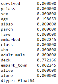
Now, let’s see the fraction of null values in each of the columns in this dataset. Run the following script:

dataset.isnull().mean()

Output:

The above output shows that 19% of the data in the age column is missing, whereas 0.2% of the data is missing from the embarked column. Also, 77% of the data in the deck column is missing!

Missing data can be broadly categorized into two types: Numeric Missing Data and Categorical Missing Data. Based on the type of missing data, different data handling techniques are used. Let’s first see how to handle numeric missing data.

Handling Numerical Missing values

Numeric data, as the name suggests, is data consisting of numbers, like the age of a passenger or price of a ticket.

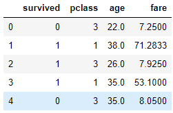
Let’s filter some of the numeric columns from the Titanic dataset and display the first five rows of the filtered data. Execute the following script:

filtered_data  = dataset[["survived", "pclass", "age", "fare"]]
filtered_data.head()

Output:

In the next sections, we’ll finally show you some of the techniques used to impute the numeric data, or replace the missing data with substituted data.

Mean and Median Imputation

In the mean and median imputation, the missing values in the dataset are either replaced by the mean or median of the remaining values.

Let’s find the mean and median values from the existing values in the age column.

median_age = filtered_data.age.median()
print(median_age)

mean_age = filtered_data.age.mean()
print(mean_age)

Output:

28.0
29.69911764705882

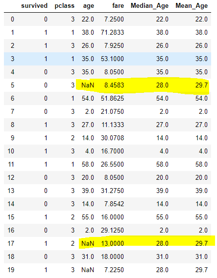
The following script creates two columns: Median_Age and Mean_Age. In the Median_Age column, the missing values in the age column are replaced by the median of the remaining values. The Pandas fillna method makes this really simple. Similarly, the Mean_Age column replaces missing values with the mean of the remaining values.

filtered_data['Median_Age'] = filtered_data.age.fillna(median_age)

filtered_data['Mean_Age'] = filtered_data.age.fillna(mean_age)

filtered_data['Mean_Age']  = np.round(filtered_data['Mean_Age'], 1)

filtered_data.head(20)

Output:

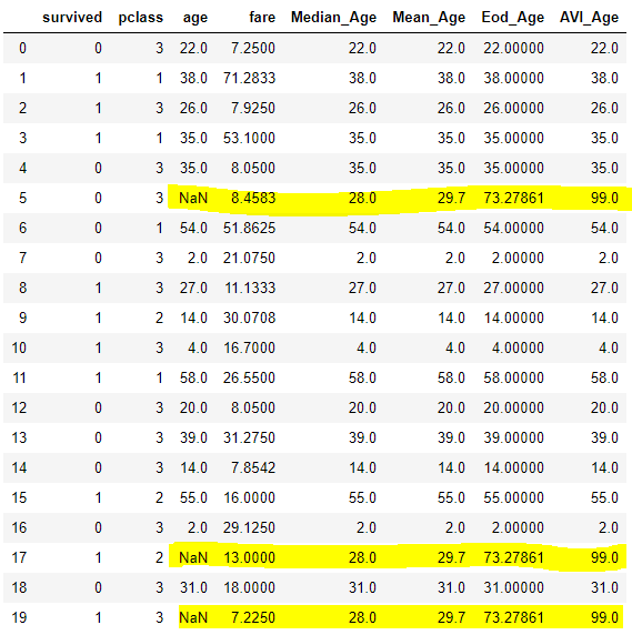
From the output above, you can see that for the rows where the age column contains null values, the Median_age and Mean_Age columns, respectively contain the median and mean of the remaining values.

End of Distribution Imputation

In the “end of distribution imputation” technique, missing values are replaced by a value that exists at the end of the distribution. To find the end of distribution value, you simply add the mean value with the three positive standard deviations. This technique is ideal for data that closely models a normal distribution, since three standard deviations contain ~99.7% of the data, according to the empirical rule.

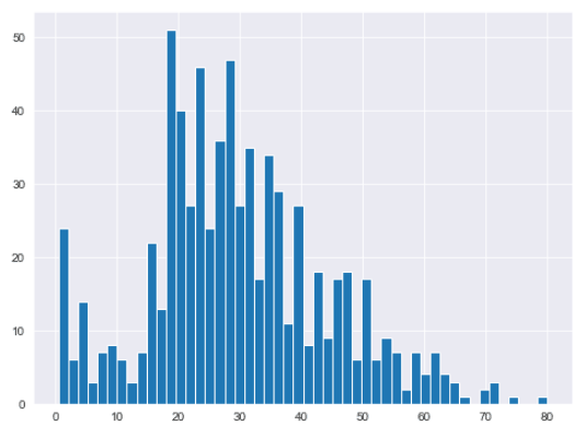
This section shows how to use the end of distribution imputation for the age column. Let’s first plot a histogram for the age column.

plt.rcParams["figure.figsize"] = [8,6]
sns.set_style("darkgrid")

filtered_data.age.hist(bins=50)

Output:

It’s clearly not a perfect normal distribution, but the end of distribution value should occur at the end of the distribution, somewhere between 70 and 80.

The following script finds the end of distribution value.

end_distribution_val = filtered_data.age.mean() + 3 * filtered_data.age.std()
print(end_distribution_val)

Output:

73.27860964406095

The end of distribution value is 73.27 for the age column. The following script creates a new column Eod_Age where missing values in the age column are replaced by the end of distribution value, 73.27.

filtered_data['Eod_Age'] = filtered_data.age.fillna(end_distribution_val)

filtered_data.head(20)

Output:

The highlighted rows in the above output shows how the null or missing values in the age column have been replaced by 73.27 in the Eod_Age column.

Arbitrary Value imputation

In arbitrary value imputation, you simply replace the null values by some arbitrary value. The arbitrary value should not be present in the dataset and should be quite different from the existing values. A common choice for arbitrary value is any combination of 9s, like 99,9999. Alternately, in cases where all the values in a column are positive, you can choose -1 as an arbitrary value. The following script replaces missing values with an arbitrary value of 99.

filtered_data['AVI_Age'] = filtered_data.age.fillna(99)

filtered_data.head(20)

Output:

Get Our Python Developer Kit for Free

I put together a Python Developer Kit with over 100 pre-built Python scripts covering data structures, Pandas, NumPy, Seaborn, machine learning, file processing, web scraping and a whole lot more - and I want you to have it for free. Enter your email address below and I'll send a copy your way.

Handling Missing Categorical Data

Categorical data is the type of data where values represent a certain category instead of numbers. For example gender of a person, the city where a person is from, whether or not a person is smoker, the nationality of a person, etc.

Recall the embark_town column and the age column have missing data in our Titanic dataset. You may be wondering why we’re talking about the age column since it’s clearly numeric and not categorical, but we’ll explain in the next section. Let’s filter both these columns.

filtered_data  = dataset[["embark_town", "age", ]]

filtered_data.isnull().mean()

Output:

embark_town    0.002245
age            0.198653
dtype: float64

Again, the output shows that 19% of the data in the age column is missing while 0.2% of the data is missing from embark_town column.

Frequent Category Imputation

In frequent category imputation, the missing categorical values are replaced by the most frequently occurring value. The most frequently occurring value is called the mode.

To find the most frequently occurring value in a column, use the mode() function. The following script finds the most frequently occurring category in the embark_town column.

station = filtered_data.embark_town.mode()[0]
print(station)

Output:

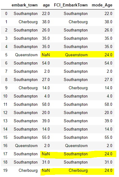
Southampton

The output shows that Southampton is the most frequently occurring category in the embark town column.

The following script replaces the missing value in the embark_town column by the value in the station variable (Southampton).

filtered_data['FCI_EmbarkTown'] = filtered_data.embark_town.fillna(station )
filtered_data.head(20)

Frequent category imputation can also be used to replace missing values in a numerical column. The mode of values in a numeric column is similar to the most frequently occurring category in a categorical column. Let’s find mode of the values in the age column.

mode_age = filtered_data.age.mode()[0]
print(mode_age)

Output:

24.0

The mode of the age column is 24. The following script creates a column mode_Age which contains mode values in place of missing values from the age column. The variable mode_age is used to add the value 24.0 to the new column.

filtered_data['mode_Age'] = filtered_data.age.fillna(mode_age)

filtered_data.head(20)

Output:

Missing Value Imputation

In missing value imputation, you simply replace a missing categorical value by a value that doesn’t exist in the column. You can give any name to the missing value. The following script replaces missing values in the embark_town column by a new category called “Missing”.

filtered_data['MVI_EmbarkTown'] = filtered_data.embark_town.fillna("Missing")

filtered_data.head(20)

To prove the missing value imputation technique worked in the above Python code, let’s filter the rows where embark_town column contains missing values.

filtered_data1 = filtered_data[filtered_data["embark_town"].isna()]
filtered_data1.head()

Output:

The output shows our new MVI_EmbarkTown column contains “Missing” as a new category for the missing values in the embark_town column. Meanwhile, the FCI_EmbarkTown column contains the most frequently occurring category we added earlier.

Once you’re finished imputing all the missing values in your datasets, you’re ready to train your machine learning algorithm. TensorFlow 2.0 is a great tool for training both regression models and classification models

For more Python data manipulation techniques like this, please join us using the form below:

Get Our Python Developer Kit for Free

I put together a Python Developer Kit with over 100 pre-built Python scripts covering data structures, Pandas, NumPy, Seaborn, machine learning, file processing, web scraping and a whole lot more - and I want you to have it for free. Enter your email address below and I'll send a copy your way.