Effective detection of leaf diseases is crucial in plant pathology as it enables farmers and growers to identify and treat affected plants promptly. One of the most efficient automation methods for this task is the utilization of Convolutional Neural Networks (CNNs). These machine-learning algorithms are particularly suitable for image classification, such as identifying diseases in leaf images.
This tutorial will guide you on implementing a CNN using the widely-used Python Keras library for deep learning. We’ll walk you through an example of using a CNN to classify leaf images and detect any diseases present.
Data Visualization
You can download the Plant Disease Recognition Dataset for this tutorial from Kaggle.
Once you download the dataset and unzip it into a directory (we downloaded the data in the
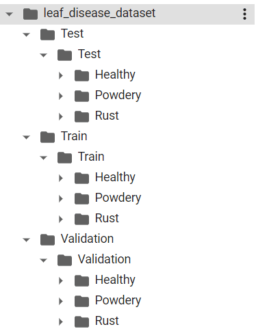
You’ll need these nested directories for our test, train, and validation sets. Each inner test, train, and validation directory contains three sub-directories Healthy, Powdery, and Rust. These directories contain the corresponding leaf images.
Our job is to train a CNN that classifies a leaf image into one of the Healthy, Powdery, or Rust categories.
The following script prints the total number of images in test, train, and validation sets.
import os

def total_files(folder_path):
  num_files = len([f for f in os.listdir(folder_path) if os.path.isfile(os.path.join(folder_path, f))])
  return num_files

train_files_healthy = "/content/leaf_disease_dataset/Train/Train/Healthy"
train_files_powdery = "/content/leaf_disease_dataset/Train/Train/Powdery"
train_files_rust = "/content/leaf_disease_dataset/Train/Train/Rust"

test_files_healthy = "/content/leaf_disease_dataset/Test/Test/Healthy"
test_files_powdery = "/content/leaf_disease_dataset/Test/Test/Powdery"
test_files_rust = "/content/leaf_disease_dataset/Test/Test/Rust"

valid_files_healthy = "/content/leaf_disease_dataset/Validation/Validation/Healthy"
valid_files_powdery = "/content/leaf_disease_dataset/Validation/Validation/Powdery"
valid_files_rust = "/content/leaf_disease_dataset/Validation/Validation/Rust"

print("Number of healthy leaf images in training set", total_files(train_files_healthy))
print("Number of powder leaf images in training set", total_files(train_files_powdery))
print("Number of rusty leaf images in training set", total_files(train_files_rust))

print("========================================================")

print("Number of healthy leaf images in test set", total_files(test_files_healthy))
print("Number of powder leaf images in test set", total_files(test_files_powdery))
print("Number of rusty leaf images in test set", total_files(test_files_rust))

print("========================================================")

print("Number of healthy leaf images in validation set", total_files(valid_files_healthy))
print("Number of powder leaf images in validation set", total_files(valid_files_powdery))
print("Number of rusty leaf images in validation set", total_files(valid_files_rust))
Output:
Number of healthy leaf images in training set 458
Number of powder leaf images in training set 430
Number of rusty leaf images in training set 434

========================================================

Number of healthy leaf images in test set 50
Number of powder leaf images in test set 50
Number of rusty leaf images in test set 50

========================================================

Number of healthy leaf images in validation set 20
Number of powder leaf images in validation set 20
Number of rusty leaf images in validation set 20
Let’s see what a healthy leaf image looks like. The following script displays one of the healthy leaf images from the training set.
from PIL import Image
import IPython.display as display

image_path = '/content/leaf_disease_dataset/Train/Train/Healthy/800edef467d27c15.jpg'

with open(image_path, 'rb') as f:
    display.display(display.Image(data=f.read(), width=500))
Output:

And the following script displays a leaf image with rust on the leaf.
image_path = '/content/leaf_disease_dataset/Train/Train/Rust/80f09587dfc7988e.jpg'

with open(image_path, 'rb') as f:
    display.display(display.Image(data=f.read(), width=500))
Output:
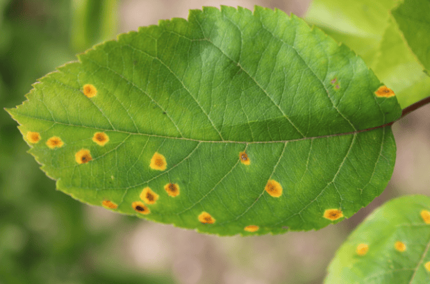
Alright, now that we know what we’re looking for, let’s work on training our image classification model with a CNN.
Training Neural Network Model for Leaf Disease Detection
In this section, you’ll see the steps required to train and evaluate a convolutional neural network for leaf disease detection.
Preparing Training Data
CNN models can be significantly slower when trained on raw input images. A good approach is to preprocess your input images to reduce their size. You can also apply transformations on the training images to increase the quantity and variety of training images.
In addition, running a Keras model on large batches of input images can result in resource exhaustion. It’s convenient to train your Keras models on smaller batches of data.
The keras.preprocessing.image.ImageDataGenerator class allows you to preprocess input images. The class also allows you to train Keras models in smaller batches.
The following script creates ImageDataGenerators objects for our training and test sets. We rescale our training images and apply shear and zoom transformations. For our test images, we’ll only apply scaling.
from keras.preprocessing.image import ImageDataGenerator

train_datagen = ImageDataGenerator(rescale=1./255, shear_range=0.2, zoom_range=0.2, horizontal_flip=True)
test_datagen = ImageDataGenerator(rescale=1./255)
The following script creates data generators for our training and validation sets.
The flow_from_directory() method tells the model to fetch our training and validation images from specified directories. Here, you can also set the target size (225 x 225) of the input images and the batch size (32) for model training. Since we have more than two classes, we use the categorical class mode.
We will train our model on the train set generators, and validate the model performance on the validation generator. For evaluating the model, we’ll create a test data generator, which you will see later.
train_generator = train_datagen.flow_from_directory('/content/leaf_disease_dataset/Train/Train',
                                                    target_size=(225, 225),
                                                    batch_size=32,
                                                    class_mode='categorical')

validation_generator = test_datagen.flow_from_directory('/content/leaf_disease_dataset/Validation/Validation',
                                                        target_size=(225, 225),
                                                        batch_size=32,
                                                        class_mode='categorical')
Output:
Found 1322 images belonging to 3 classes.
Found 60 images belonging to 3 classes.
Designing the Convolutional Neural Network Architecture in Keras
Designing convolutional neural network models with Keras is simple. Everything remains the same as the densely connected neural network. For convolutions, you simply have to add convolution and max pooling layers. You can add convolution and pooling layers using the keras.layers.Conv2D class and keras.layers.MaxPooling2D classes, respectively.
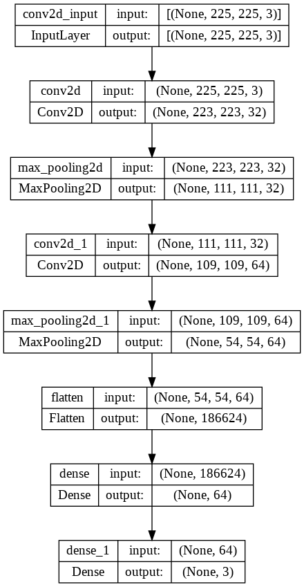
The following script defines a convolutional neural network with two convolution layers, one flatten layer and two dense layers. Notice that the number of neurons in the final dense layers is 3, corresponding to the number of classes in our dataset.
If you’re curious, here’s an excellent article describing the theory behind convolutional neural networks.
from keras.models import Sequential
from keras.layers import Conv2D, MaxPooling2D, Flatten, Dense


model = Sequential()
model.add(Conv2D(32, (3, 3), input_shape=(225, 225, 3), activation='relu'))
model.add(MaxPooling2D(pool_size=(2, 2)))
model.add(Conv2D(64, (3, 3), activation='relu'))
model.add(MaxPooling2D(pool_size=(2, 2)))
model.add(Flatten())
model.add(Dense(64, activation='relu'))
model.add(Dense(3, activation='softmax'))
Okay, now that we’ve done that, we must compile the model before training it. You can do so using the compile() method. We use the Adam optimizer and the categorical cross entropy loss function for model training. You can use other optimizers if you want but the Adam optimizer works the best in most cases.
model.compile(optimizer='adam', loss='categorical_crossentropy', metrics=['accuracy'])Keras is neat because it lets you visualize your model, if that’s something you’re interested in. for example, we can see our CNN model architecture using the keras.utils.plot_model() method below:
from keras.utils import plot_model
plot_model(model, to_file='model.png', show_shapes=True)
Output:
Training the Model
To train a CNN in Keras, you call the fit() method and pass it the train and validation generators. The batch_size here corresponds to the number of steps before the neural network weights are updated within an epoch. We train the model for 5 epochs (iterations), but you can try more epochs if you want.
history = model.fit(train_generator,
                    batch_size=16,
                    epochs=5,
                    validation_data=validation_generator,
                    validation_batch_size=16
                    )
It’ll take a while to run, but once it’s finished, our output shows our model achieves an accuracy of 85% on the validation set.
Output:
Epoch 1/5
42/42 [==============================] - 186s 4s/step - loss: 1.1745 - accuracy: 0.6263 - val_loss: 0.6446 - val_accuracy: 0.7167
Epoch 2/5
42/42 [==============================] - 181s 4s/step - loss: 0.4320 - accuracy: 0.8192 - val_loss: 0.4846 - val_accuracy: 0.8333
Epoch 3/5
42/42 [==============================] - 181s 4s/step - loss: 0.3357 - accuracy: 0.8812 - val_loss: 0.4576 - val_accuracy: 0.8667
Epoch 4/5
42/42 [==============================] - 181s 4s/step - loss: 0.2661 - accuracy: 0.9077 - val_loss: 0.5161 - val_accuracy: 0.8000
Epoch 5/5
42/42 [==============================] - 181s 4s/step - loss: 0.2511 - accuracy: 0.9153 - val_loss: 0.3561 - val_accuracy: 0.8500
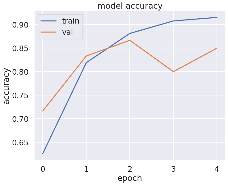
Let’s plot our validation accuracy against the number of epochs. The output shows that the best accuracy is achieved after the third epoch.
from matplotlib import pyplot as plt
from matplotlib.pyplot import figure

import seaborn as sns
sns.set_theme()
sns.set_context("poster")

figure(figsize=(10, 8), dpi=80)

plt.plot(history.history['accuracy'])
plt.plot(history.history['val_accuracy'])
plt.title('model accuracy')
plt.ylabel('accuracy')
plt.xlabel('epoch')
plt.legend(['train', 'val'], loc='upper left')
plt.show()
Output:
Evaluating the Model and Making Predictions
A validation set is ideal for testing your neural network and fine-tuning your model parameters. The final model evaluation should be performed on an unseen test set. Let’s do that.
The following script creates a data generator for the test set. It then passes the test data generator to the evaluate() method to evaluate the model performance on the test set.
test_generator = test_datagen.flow_from_directory('/content/leaf_disease_dataset/Test/Test',
                                                        target_size=(225, 225),
                                                        batch_size=32,
                                                        class_mode='categorical')

model.evaluate(test_generator)
Output:
The output below shows that our model achieves an accuracy of 88% on the unseen test set, which is very impressive for a basic CNN architecture.
Found 150 images belonging to 3 classes.
5/5 [==============================] - 18s 4s/step - loss: 0.3158 - accuracy: 0.8800
[0.31578144431114197, 0.8799999952316284]
To make predictions on a new single image, you can use the predict() method of the trained model.
You’ll need to preprocess your input image and convert it to the image format used for training the model. Recall that we resized our input images to 225 x 225 and rescaled them by dividing pixel values by 255. The following script defines a function that can preprocess your input images.
For example, We preprocessed a a random image from the rust folder in the test, but you can use any leaf photo you’ve taken if you want to see how it performs.
from tensorflow.keras.utils import load_img, img_to_array
import numpy as np

def preprocess_image(image_path, target_size=(225, 225)):
    # load image
    img = load_img(image_path, target_size=target_size)

    # convert to array and preprocess
    x = img_to_array(img)
    x = x.astype('float32') / 255.
    x = np.expand_dims(x, axis=0)

    return x

x = preprocess_image('/content/leaf_disease_dataset/Test/Test/Rust/82f49a4a7b9585f1.jpg')
The following script makes predictions on the single test image using our pre-processed image,
predictions = model.predict(x)
predictions[0]
Output:
1/1 [==============================] - 0s 15ms/step
array([2.9100770e-02, 4.9777434e-04, 9.7040141e-01], dtype=float32)
You can see that index 2 has the highest prediction probability (0.970). We need to convert the predicted index back to the original label value.
To get the inverse mapping of class labels to class indices from a keras.preprocessing.image.ImageDataGenerator object used in training, you can use the class_indices attribute and invert the dictionary using a dictionary comprehension.
labels = train_generator.class_indices
labels = {v: k for k, v in labels.items()}
labels
Output:
{0: 'Healthy', 1: 'Powdery', 2: 'Rust'}Finally, you can retrieve the label with the highest predicted probability using the following script:
predicted_label = labels[np.argmax(predictions)]
print(predicted_label)
Output:
RustYou can see that index 2 corresponds to the label rust, which shows that our model correctly predicted that the leaf in the input image is rusty. How cool is that?
