With the availability of huge amounts of data and high performance computing hardware, more and more companies are now relying on machine learning algorithms to make business decisions. Machine learning algorithms, or at least the ones we’ll be describing today, try to make predictions about the future based on historical data. Machine learning algorithms are divided into two types: supervised and unsupervised machine learning.
Supervised machine learning algorithms are further divided into classification and regression models. In regression models, the goal is to predict a continuous value like the price of a house or the score of a student on a particular exam. In classification models, the task is to predict one of the several predefined labels for a record. For instance, whether or not a tumor is malignant or whether or not a bank note is fake. We’ve talked about using TensorFlow 2.0 for both regression and classification tasks before, but this tutorial will be a little different. I encourage you to read these tutorials before diving into this one, since they give some good background on general machine learning terms, like batch size and epochs.
In this tutorial, we’ll show you examples for solving classification problems with Python’s Scikit-learn library which is one of the most commonly used libraries for machine learning in Python.
In the first problem, you’ll see how to predict whether or not a bank customer will churn in the future. In the second problem, you’ll see how to predict a car’s condition based on different attributes such as the car’s price, maintenance cost, number of doors, etc.
Installing Required Libraries
Before we proceed further, we need to install the Python libraries needed to run the scripts in this tutorial. Execute the following commands on your terminal to download the required libraries.
$ pip install numpy
$ pip install pandas
$ pip install matplotlib
$ pip install scikit-learn
Predicting Customer Churn
In our first task, we’ll predict customer churn based on several attributes such as the customer’s location, credit card history, and bank balance.
Importing the Dataset
Before importing our dataset, execute the following script to import the libraries required to handle the dataset in Python.
import numpy as np
import matplotlib.pyplot as plt
import pandas as pd
The dataset for this problem can be downloaded freely from this kaggle link. Download the dataset locally and then execute the following command to load the data into your Python application. You’ll need to update the file path to match where you saved your file.
dataset = pd.read_csv(r'C:/Datasets/customer_data.csv')
dataset.head()
Output:
The output shows that the dataset has 14 columns. Based on the first 13 columns, we have to predict the value in the exited column i.e. whether or not the customer will exit the bank within 6 months after the data for the first 13 columns is recorded.
Our dataset doesn’t have any missing values, but yours may be different. If the dataset you’re working with contains missing values, read our tutorial on imputing missing values before training your machine learning algorithm.
Data Preprocessing
Some of the columns in our dataset are totally random and do not help us indicate whether or not a customer will leave the bank. For instance, the RowNumber, CustomerId and Surname columns do not play any part in a customer’s decision to churn or stay with a bank. Let’s remove these three columns from our dataset.
dataset = dataset.drop(['RowNumber', 'CustomerId', 'Surname'], axis=1)Algorithms in Scikit-learn library work with numerical features. Some of the features in our dataset are categorical, like Geography and Gender which contain textual data. To convert textual features into numeric features, we can use the one-hot encoding technique. In one-hot encoding, a new column is created for each unique value in the original column. The integer 1 is added to one of the new columns that corresponds to the original value. In the remaining columns 0s are added. This is best explained with the help of an example.
Let’s first remove the categorical columns Geography and Gender from our dataset and create a
temp_dataset = dataset.drop(['Geography', 'Gender'], axis=1)Next, let’s use Pandas get_dummies()method to convert the categorical columns into numeric columns. Look at the following script.
onehot_geo = pd.get_dummies(dataset.Geography)
onehot_gen = pd.get_dummies(dataset.Gender)
onehot_geo.head()
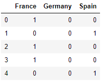
The above script prints the newly one-hot encoded columns for the original Geography and Gender columns. Here’s what the output for Geography looks like:
Output:
The output shows that 1 has been added in the column for France in the first row, while the Germany and Spain columns contain 0. This is because in the original Geography column, the first row contained France.
Now we’re going to take these new columns and add them to our
final_dataset = pd.concat([temp_dataset, onehot_geo, onehot_gen], axis=1)Dividing the Data into Training and Test Sets
Next, we need to divide our dataset into training and test sets. The training set will be used to train the machine learning classifiers, while the test set will be used to evaluate the performance of our classifier.
Before dividing the data into training and test set, we need to divide the data into features and labels. The feature set contains independent variables, and the label set contains dependent variable or the labels that you want to predict. The following script divides the dataset into feature set
X =  final_dataset.drop(['Exited'], axis=1).values
y = final_dataset['Exited'].values
From here, we can further divide our data into training and test sets:
from sklearn.model_selection import train_test_split
X_train, X_test, y_train, y_test = train_test_split(X, y, test_size = 0.2, random_state = 0)
Training and Evaluating the Machine Learning Classifier
We are now ready to train the machine learning models on our dataset. There are several machine learning classifiers available in the Scikit-learn library. However, we will be using the Random Forest classifier which is one of the most powerful machine learning classifiers.
We can train our algorithm using the RandomForestClassifier class from the sklearn.ensemble module. To train the algorithm we need to pass the training features and labels to the fit() method of the RandomForestClassifier class. To make predictions on the test set, the predict() method is used as shown below:
from sklearn.ensemble import RandomForestClassifier
clf = RandomForestClassifier(n_estimators=200, random_state=0)
clf.fit(X_train, y_train)
y_pred = clf.predict(X_test)
Once the model is trained, you can use a variety of evaluation metrics to measure the algorithm’s performance on your test set. Some of the most commonly used measures are accuracy, confusion matrix, precision, recall and F1. The following script calculates these values for our model when the model is evaluated on our test set.
from sklearn.metrics import classification_report, accuracy_score
print(classification_report(y_test,y_pred))
print(accuracy_score(y_test, y_pred ))
Output:
precision    recall  f1-score   support

      0       0.89      0.96      0.92      1595
      1       0.76      0.52      0.62       405

accuracy                           0.87      2000
macro avg       0.82      0.74      0.77      2000
weighted avg       0.86      0.87      0.86      2000

0.8695
The output shows that our model achieves an accuracy of 86.95% on the test set which is pretty good.
In the next section, you will see another example of how to perform classification with Python’s Scikit-learn library.
Predicting Car Conditions
Knowing how good a car is before you make a purchase decision can save you lots of pain in the future. Believe it or not, machine learning can help you here, too. We can develop a machine learning algorithm capable of predicting a car’s condition based on several attributes such as buying price, maintenance price, number of doors, seating capacity etc. All you need is some historical data of cars with such attributes.
Importing the Dataset
The dataset for this problem is available at this GitHub link.
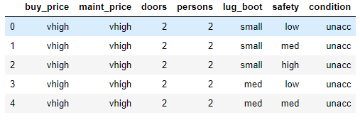
Let’s import the dataset and print its first five rows.
colnames=['buy_price', 'maint_price', 'doors', 'persons', 'lug_boot', 'safety','condition']
dataset = pd.read_csv(r'C:/Datasets/car_evaluation.csv', names=colnames, header=None)
dataset.head()
Output:
The dataset has 7 columns. Based on the first 6 columns, our task is to predict the car condition which can either be unacc (unacceptable), acc (acceptable), good and vgood (very good).
Let’s first check the type of all the columns.
Data Preprocessing
dataset.dtypesOutput:
buy_price      object
maint_price    object
doors          object
persons        object
lug_boot       object
safety         object
condition      object
dtype: object
All the columns in our dataset are of type objects. We need to convert the feature set into numeric data as we did in the case of bank customer churn. Just like before, we’re going to use one-hot encoding again to do this. The following script removes the categorical feature columns from our dataset and stores the condensed dataset in
temp_dataset = dataset.drop(['buy_price', 'maint_price', 'doors', 'persons', 'lug_boot', 'safety'] , axis=1)Once the categorical columns are removed, run this script to perform one-hot encoding on the categorical columns.
onehot_buy = pd.get_dummies(dataset.buy_price, prefix = 'buy_price')
onehot_maint = pd.get_dummies(dataset.maint_price, prefix = 'maint_price')

onehot_doors = pd.get_dummies(dataset.doors, prefix = 'doors')
onehot_persons = pd.get_dummies(dataset.persons, prefix = 'persons')

onehot_lug_boot = pd.get_dummies(dataset.lug_boot, prefix = 'lug_boot')
onehot_safety = pd.get_dummies(dataset.safety, prefix = 'safety')
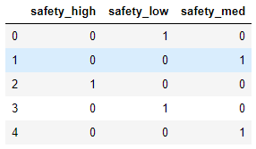
Now, if you look at the one-hot encoded safety column, you should see the following output.
onehot_safety.head()Output:
The final dataset can be created by concatenating the one-hot encoded columns with our condensed dataset where we removed the categorical columns,
final_dataset = pd.concat([onehot_buy, onehot_maint, onehot_doors, onehot_persons, onehot_lug_boot, onehot_safety, temp_dataset] , axis=1)Dividing Data into Training and Test Sets
The remaining steps are similar to our bank customer churn problem. We first divide our data into the features and labels set.
X =  final_dataset.drop(['condition'], axis=1).values
y = final_dataset['condition'].values
And then we can divide our data into the training and test set as shown below:
from sklearn.model_selection import train_test_split
X_train, X_test, y_train, y_test = train_test_split(X, y, test_size = 0.2, random_state = 0)
Training and Evaluating the Machine Learning Classifier
We can again train our algorithm (model) using the RandomForestClassifier class from the sklearn.ensemble module as shown below:
from sklearn.ensemble import RandomForestClassifier
clf = RandomForestClassifier(n_estimators=400, random_state=0)
clf.fit(X_train, y_train)
y_pred = clf.predict(X_test)
Finally, the following script evaluates our model performance.
from sklearn.metrics import classification_report, accuracy_score
print(classification_report(y_test,y_pred))
print(accuracy_score(y_test, y_pred ))
Output:
precision    recall  f1-score   support

   acc       0.90      0.96      0.93        79
  good       0.87      0.76      0.81        17
 unacc       1.00      0.97      0.99       240
 vgood       0.69      0.90      0.78        10

accuracy                           0.96       346
macro avg       0.87      0.90      0.88       346
weighted avg       0.96      0.96      0.96       346

0.9595375722543352
The output shows that our model is 95.95% accurate while making predictions on the test set, which is an extremely excellent result. This model can now be used to evaluate the condition of other cars with approximately 96% accuracy.


