Using Python TensorFlow 2.0 for Classification Tasks

TensorFlow 2.0 is the latest version of Google’s TensorFlow Library for deep learning. TensorFlow 2.0 is released as a Python library, so you can use it to perform several deep learning tasks from within your Python applications.

In this tutorial, we’ll show you how to perform classification using the TensorFlow 2.0 library. Classification is a type of supervised machine learning task where you assign one or more predefined labels to data instances. Specifically, this tutorial develops a deep learning tool to classify iris plants based on their physical properties. This is a great example of how you can use Python’s TensorFlow 2.0 library for data classification tasks. Let’s show you how it works!

Note: All the codes in this article are compiled with the Jupyter Notebook.

TensorFlow 2.0 Installation

To install the TensorFlow 2.0 library, you can use pip installer. The following command installs the TensorFlow 2.0 library:

$ pip install tensorflow

If you have an old version of TensorFlow already installed, you can update your TensorFlow to version 2.0 via the following command:

pip install --upgrade tensorflow

The other libraries you will need to install in order to execute the scripts in this tutorial are Pandas, Seaborn, NumPy, Scikit-Learn, and Matplotlib. The following script installs these libraries:

pip install matplotlib
pip install seaborn
pip install pandas
pip install NumPy
pip install scikit-learn

Import Required Libraries

Before we actually perform classification with TensorFlow 2.0, let’s first import the seaborn, matplotlib, pandas and TensorFlow modules that we are going to need in this tutorial:

import seaborn as sns
import pandas as pd
import numpy as np

from tensorflow.keras.layers import Input, Dense, Dropout, Activation
from tensorflow.keras.models import Model

You’re going to see how we use each of these libraries a little later in this tutorials.

You can check the version of the TensorFlow installed on your system by executing the following Python Script:

tf.__version__

As of the date of this publication, you should see “2.0.0” in the output.

Importing and Preprocessing the Dataset

We will be performing classification on the Iris dataset. You don’t need to download the Iris dataset since it comes prebuilt with the Seaborn library. Execute the following script to import and display the first five rows of the dataset:

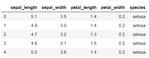
dataset = sns.load_dataset('iris')
dataset.head()

Output:

The dataset contains five columns: sepal_length, sepal_width, petal_length, petal_width, and species. Based on the information in the first four columns, which is also known as the feature set, we want to use TensorFlow to predict the species of the iris plant.

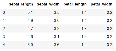
To do this, we’ll divide our dataset into features and label sets. The feature set contains the first four columns, which describe the plant. The label set contains the data from the species column. The following script divides the data into features and label sets. The script also prints the first 5 records from the feature set.

X = dataset.drop(['species'], axis=1)
y = pd.get_dummies(dataset.species, prefix='output')
X.head()

Output:

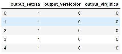
In the same way, we can print the first five rows from the label set.

y.head()

Output:

You may notice that originally the labels column i.e. species contained string values. But here in the above output, the label set has three columns where column names correspond to actual values in the species column. This is called one hot encoding of categorical features. Since the TensorFlow library only works with numbers, we have to convert the string type data into numbers. One hot encoding is one of several approaches used to convert string data to numbers.

Next, we need to convert our pandas dataframes into NumPy array since both Scikit learn and TensorFlow libraries accept inputs in the form of Numpy arrays.

X = X.values
y = y.values

Get Our Python Developer Kit for Free

I put together a Python Developer Kit with over 100 pre-built Python scripts covering data structures, Pandas, NumPy, Seaborn, machine learning, file processing, web scraping and a whole lot more - and I want you to have it for free. Enter your email address below and I'll send a copy your way.

Dividing Data into Training and Test assets

In machine learning and deep learning, data is divided into the training and test sets. The training set is used to train a deep learning model while the test set is used to evaluate the performance of the trained model. The following script divides the data into 80% training set and 20% test set. This ratio is defined by the test_size attribute of the train_test_split() function as shown below:

from sklearn.model_selection import train_test_split
X_train, X_test, y_train, y_test = train_test_split(X, y, test_size=0.20, random_state=39)

Next, before we train our deep learning model, we need to scale our data. Scaling can be useful since the magnitude of data in different columns can vary hugely, and therefore it is a good practice to scale the dataset so that all the columns have similar data scales.

from sklearn.preprocessing import StandardScaler
sc = StandardScaler()
X_train = sc.fit_transform(X_train)
X_test = sc.transform(X_test)

Defining TensorFlow models

So far all we’ve done is preprocess our data. All this is necessary before we can even begin defining our TensorFlow model. In this example, our TensorFlow model will be simple. It will consist of a densely connected neural network. If you are not familiar to neural networks, check out this link.

Our neural network will contain an input layer, three hidden layers and one output layer. The hidden layers will be densely connected. The first layer contains 100 neurons, the second hidden layer contains 50 neurons, and the third hidden layer contains 25 neurons. You can play around with these values to see if you get better results.

input_1 = Input(shape=(X_train.shape[1],))
l1 = Dense(100, activation='relu')(input_1)
l2 = Dense(50, activation='relu')(l1)
l3 = Dense(25, activation='relu')(l2)
output_1 = Dense(y_train.shape[1], activation='softmax')(l3)

model = Model(inputs = input_1, outputs = output_1)
model.compile(loss='categorical_crossentropy', optimizer='adam', metrics=['acc'])

The above script creates our neural network model. To compile the model, the compile() method is used. To connect previous layer to the next layer, you simply have to add the previous layer name inside the parenthesis that follow the next layer name.

Training and Testing the Model

Once the model is created, you have can train it by simply calling the fit() method. The method requires you pass it the training set (i.e. the training features and labels, the batch size and the number of epochs). The batch size refers to the number of records processed at once and the epochs refers to the number of iterations for which the model will be trained on the complete dataset. Here’s how you call the .fit() method:

history = model.fit(X_train, y_train, batch_size=4, epochs=20, verbose=1, validation_split=0.20)

While the model is being trained, you can see the accuracy obtained after each epoch. The output below only shows the results from the first 5 epochs, but you should see result from all 20 epochs.

Output:

Train on 96 samples, validate on 24 samples
Epoch 1/20
96/96 [==============================] - 1s 7ms/sample - loss: 0.8962 - acc: 0.5938 - val_loss: 0.8076 - val_acc: 0.7500
Epoch 2/20
96/96 [==============================] - 0s 457us/sample - loss: 0.6085 - acc: 0.8229 - val_loss: 0.6318 - val_acc: 0.7917
Epoch 3/20
96/96 [==============================] - 0s 603us/sample - loss: 0.4415 - acc: 0.8438 - val_loss: 0.5418 - val_acc: 0.7500
Epoch 4/20
96/96 [==============================] - 0s 530us/sample - loss: 0.3344 - acc: 0.8438 - val_loss: 0.4666 - val_acc: 0.7500
Epoch 5/20
96/96 [==============================] - 0s 364us/sample - loss: 0.2608 - acc: 0.8854 - val_loss: 0.4175 - val_acc: 0.8333

Once the model is trained, the final step is to evaluate the model performance on your actual test set. To do so, you need to call the evaluate() method on the model class and pass it your test features and test labels.

score = model.evaluate(X_test, y_test, verbose=1)

print("Test Accuracy:", score[1])

Output:

0s 5ms/sample - loss: 0.1586 - acc: 0.9667
Test Accuracy: 0.96666664

The output shows our TensorFlow 2.0 model accurately categorized 96.67% of the iris data in our test set based solely on the physical features of the plant. That’s impressive, isn’t it?

Complete Code

To help you with your own Python TensorFlow 2.0 projects, here is the complete code we used to perform deep learning classification in this tutorial:

import seaborn as sns
import pandas as pd
import numpy as np

from tensorflow.keras.layers import Input, Dense, Dropout, Activation
from tensorflow.keras.models import Model

dataset = sns.load_dataset('iris')
dataset.head()

X = dataset.drop(['species'], axis=1)
y = pd.get_dummies(dataset.species, prefix='output')


X.head()

y.head()

X = X.values
y = y.values

from sklearn.model_selection import train_test_split
X_train, X_test, y_train, y_test = train_test_split(X, y, test_size=0.20, random_state=39)

from sklearn.preprocessing import StandardScaler
sc = StandardScaler()
X_train = sc.fit_transform(X_train)
X_test = sc.transform(X_test)

input_1 = Input(shape=(X_train.shape[1],))
l1 = Dense(100, activation='relu')(input_1)
l2 = Dense(50, activation='relu')(l1)
l3 = Dense(25, activation='relu')(l2)
output_1 = Dense(y_train.shape[1], activation='softmax')(l3)

model = Model(inputs = input_1, outputs = output_1)
model.compile(loss='categorical_crossentropy', optimizer='adam', metrics=['acc'])

print(model.summary())

history = model.fit(X_train, y_train, batch_size=4, epochs=20, verbose=1, validation_split=0.20)

score = model.evaluate(X_test, y_test, verbose=1)

print("Test Accuracy:", score[1])

Get Our Python Developer Kit for Free

I put together a Python Developer Kit with over 100 pre-built Python scripts covering data structures, Pandas, NumPy, Seaborn, machine learning, file processing, web scraping and a whole lot more - and I want you to have it for free. Enter your email address below and I'll send a copy your way.