In this article, we will explore how to solve classification and regression problems using deep learning in PyTorch, a popular deep learning framework. Specifically, we will focus on developing PyTorch models to solve classification and regression problems on tabular datasets. By the end of this tutorial, you will have a solid understanding of how to build and train PyTorch models for classification and regression tasks and you’ll be able to apply these techniques to your own projects.
Solving Classification Problems with PyTorch
In this section, we will solve a classification problem using PyTorch. Specifically, we will be working with the well-known iris dataset, which contains information about different species of iris plants. The goal is to classify each observation into one of three different species (setosa, versicolor, or virginica) based on the measurements of the sepal length, sepal width, petal length, and petal width.
To solve this classification problem, we will first preprocess the data and split it into training and testing sets. Then, we will define our PyTorch model, including the layers, activation functions, and loss function. After defining the model, we will train it on the training data and evaluate its performance on the testing data using various classification metrics.
Import Required Libraries
First, we need to import the necessary libraries. We’ll be using PyTorch and Pandas in this tutorial so make sure you have those installed. Later, we will also import the Sklearn library for splitting our data into train/test splits and for importing evaluation metrics.
import torch
import torch.nn as nn
import torch.optim as optim
import pandas as pd
Importing and Preprocessing the Dataset
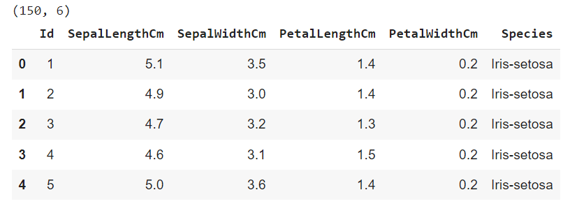
The following code loads the CSV file containing the Iris dataset into a pandas dataframe using the read_csv() function. The shape attribute of the dataframe is then printed, which returns the number of rows and columns in the dataframe. Finally, the first few rows of the dataframe are printed using the head function.
dataset = pd.read_csv('/content/Iris.csv')
print(dataset.shape)
dataset.head()
Output:
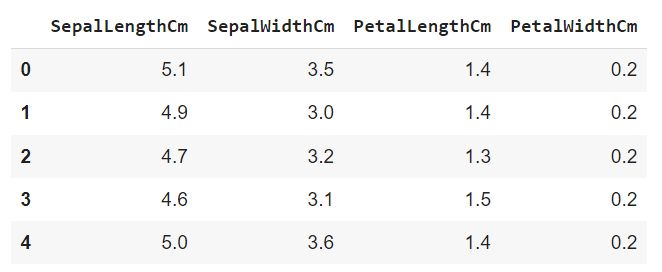
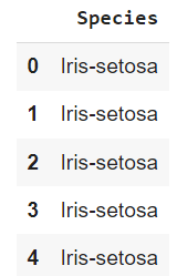
Next, we divide the dataset into features and labels. The feature set will consist of all the columns except the “Id” and “Species” column. The label set will contain values from the “Species” column, as this is what we want to predict.
X = dataset.drop(["Id", "Species"], axis = 1)
X.head()
Output:
y = dataset.filter(["Species"], axis = 1)
y.head()
Output:
Before we convert our feature into a torch tensor, we extract the feature and label values from the corresponding dataframes using the values attribute.
X = X.values
y = y.values
The labels are in a string format, so we need to convert them into integers since PyTorch models expect labels in numeric format as torch tensors. The following script uses the LabelEncoder class from the sklearn.preprocessing module to convert string labels to integers.
from sklearn.preprocessing import LabelEncoder

le = LabelEncoder()
y = le.fit_transform(y)
Next, we will divide our dataset into training and test sets. We will train our PyTorch model using the training set and will evaluate the trained model on the test set.
from sklearn.model_selection import train_test_split
X_train, X_test, y_train, y_test = train_test_split(X, y, test_size=0.2, random_state=0)
Finally, we will convert our training and test set into torch tensors.
X_train = torch.tensor(X_train).float()
X_test = torch.tensor(X_test).float()
y_train = torch.tensor(y_train).long()
y_test = torch.tensor(y_test).long()
Defining a Pytorch Model for Classification
In PyTorch, models are defined as subclasses of the nn.Module class, as shown in the following script.
class Net(nn.Module):
    def __init__(self, input_size, hidden_size, num_classes):
        super(Net, self).__init__()
        self.fc1 = nn.Linear(input_size, hidden_size)
        self.relu = nn.ReLU()
        self.fc2 = nn.Linear(hidden_size, num_classes)

    def forward(self, x):
        out = self.fc1(x)
        out = self.relu(out)
        out = self.fc2(out)
        return out

model = Net(input_size=4, hidden_size=8, num_classes=3)
The Net class defined here is a simple neural network with one hidden layer, used for classification tasks.
The __init__() method initializes the layers of the network. Here, we have three layers: an input layer, a hidden layer, and an output layer. The input layer size is set to 4 since the iris dataset has four features. The hidden layer size is set to 8 in this case. You can play around with the hidden layer size. Finally, the output layer size is set to 3 to represent the three different iris plant categories.
The forward method defines the computation that happens in the neural network. The input x is passed through the layers of the network using the fc1, relu, and fc2 layers, in order. The fc1 layer performs a linear transformation on the input, relu applies the rectified linear activation function, and fc2 performs another linear transformation to produce the final output.
Finally, an instance of the Net class is created with the input size, hidden size, and number of classes set to 4, 8, and 3, respectively. This instance of the Net class represents our neural network model that we will train and use to make predictions.
Training the Model
The next step is to train the model and make predictions. To do so, we need to define the loss function and optimizer. In PyTorch, we can use the nn.CrossEntropyLoss() function as the loss function for multi-class classification problems. We will also use the Stochastic Gradient Descent (SGD) optimizer with a learning rate of 0.01 and momentum of 0.9. You can use any other optimizer, like Adam, if you want. We’ll demonstrate use of the Adam optimizer in our regression example later in this tutorial.
Next, we define the number of epochs and an empty list to store the loss values during training. Then, we loop through each epoch and perform the following steps:
- Set the gradients to zero using
optimizer.zero_grad() - Forward pass through the model using the training data using
outputs = model(X_train) - Calculate the loss between the predicted outputs and the true labels using
criterion(outputs, y_train). - Backpropagate the error through the network using
loss.backward()and store the loss values in theloss_valslist. - Update the model parameters using
optimizer.step()
At the end of each epoch, we print the current epoch number and the loss value. The .item() function is used to extract the loss value from the PyTorch tensor, and detach().numpy() is used to convert it to a NumPy array.
By the end of this loop, our model will be trained and ready to make predictions on new data.
criterion = nn.CrossEntropyLoss()
optimizer = optim.SGD(model.parameters(), lr=0.01, momentum=0.9)

num_epochs = 100

loss_vals = []

for epoch in range(num_epochs):

    optimizer.zero_grad()

    outputs = model(X_train)

    loss = criterion(outputs, y_train)

    loss.backward()

    loss_vals.append(loss.detach().numpy().item())

    optimizer.step()

    if (epoch+1) % 10 == 0:
        print(f'Epoch [{epoch+1}/{num_epochs}], Loss: {loss.item():.4f}')
Output:
Epoch [10/100], Loss: 0.9314
Epoch [20/100], Loss: 0.7158
Epoch [30/100], Loss: 0.5329
Epoch [40/100], Loss: 0.4291
Epoch [50/100], Loss: 0.3700
Epoch [60/100], Loss: 0.3272
Epoch [70/100], Loss: 0.2915
Epoch [80/100], Loss: 0.2607
Epoch [90/100], Loss: 0.2346
Epoch [100/100], Loss: 0.2126
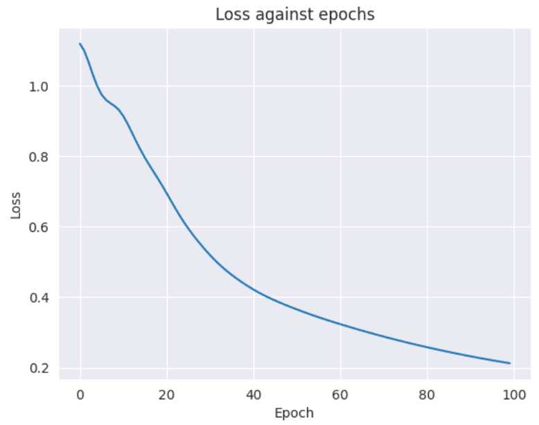
We can plot the loss to see how it decreases with each epoch. This is a good practice to help you identify any model performance anomalies.
import seaborn as sns
sns.set_style('darkgrid')
import matplotlib.pyplot as plt


indexes = list(range(len(loss_vals)))

sns.lineplot(x = indexes, y = loss_vals)

plt.xlabel('Epoch')
plt.ylabel('Loss')
plt.title('Loss against epochs')

plt.show()
Output:
Making Predictions on the Test Set
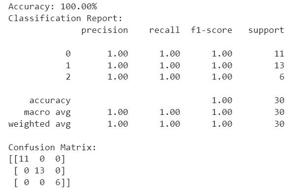
Next, we make predictions on the test set using the trained model. We start by importing the required classification metrics from the scikit-learn library. These metrics are the accuracy_score, classification_report, and confusion_matrix.
The with torch.no_grad() context manager is used to turn off gradient computation, which reduces the memory requirements and speeds up the computations.
The outputs of the model for the test set are computed using outputs = model(X_test), where X_test is the input tensor for the test set. The torch.max function is then used to extract the predicted class labels with the highest scores, which are stored in the predicted variable.
Next, the accuracy_score, classification_report, and confusion_matrix functions are used to compute the accuracy, classification report, and confusion matrix for the predicted labels and the true labels of the test set.
from sklearn.metrics import accuracy_score, classification_report, confusion_matrix

with torch.no_grad():
    outputs = model(X_test)
    _, predicted = torch.max(outputs.data, 1)

    accuracy = accuracy_score(y_test, predicted)
    report = classification_report(y_test, predicted)
    matrix = confusion_matrix(y_test, predicted)

    print(f'Accuracy: {100 * accuracy:.2f}%')
    print(f'Classification Report:\n{report}')
    print(f'Confusion Matrix:\n{matrix}')
Output:
Voila, we achieved 100% accuracy on the test set. The problem we just solved is simple, yet it conveys all the necessary steps to implement a classification model for tabular datasets in Pytorch so you should be able to recreate those steps with your own dataset to solve your own classification problem.
Solving Regression Problems with PyTorch
In this section, we will explore how to use PyTorch to solve regression problems. Specifically, we will be predicting the price per unit area of a house, using a dataset containing various features such as the transaction date, house age, distance to the nearest mass rapid transit station, number of convenience stores, latitude and longitude.
The process of solving regression problems is similar to classification problems, with the main difference being in the loss function used. While classification problems output discrete values and typically use cross-entropy loss, regression problems output continuous values and can use mean squared error loss.
In this section, we will go through the steps of preparing the data, defining and training the model, evaluating the model’s performance, and making predictions on a test set.
Importing and Preprocessing the Dataset
The following script imports the real estate dataset which is freely available on Kaggle.
dataset = pd.read_csv('/content/Real estate.csv')
print(dataset.shape)
dataset.head()
Output:
The script below divides the dataset into features and labels sets.
X = dataset.drop(["No", "Y house price of unit area"], axis = 1).values
y = dataset.filter(["Y house price of unit area"], axis = 1).values
Next we divide the dataset into training and test sets, then convert the dataset features and labels to torch tensors.
from sklearn.model_selection import train_test_split

X_train, X_test, y_train, y_test = train_test_split(X, y, test_size=0.2, random_state=0)

X_train = torch.tensor(X_train).float()
X_test = torch.tensor(X_test).float()
y_train = torch.tensor(y_train).float()
y_test = torch.tensor(y_test).float()
Defining PyTorch Model for Regression
The following script defines a PyTorch neural network model that has six fully connected layers, with input size of 6 (corresponding to six input features) and output size of 1, which means it takes a tensor of size (batch_size, 6) as input and produces a tensor of size (batch_size, 1) as output.
Notice that here the last layer has no activation function, because it is a regression problem and we want to predict continuous values.
You can add or remove some of the hidden layers to see if you get better results.
class Net(nn.Module):
    def __init__(self):

        super(Net, self).__init__()
        self.fc1 = nn.Linear(6, 256)
        self.fc2 = nn.Linear(256, 128)
        self.fc3 = nn.Linear(128, 128)
        self.fc4 = nn.Linear(128, 64)
        self.fc5 = nn.Linear(64, 32)
        self.fc6 = nn.Linear(32, 1)

    def forward(self, x):
        x = torch.relu(self.fc1(x))
        x = torch.relu(self.fc2(x))
        x = torch.relu(self.fc3(x))
        x = torch.relu(self.fc4(x))
        x = torch.relu(self.fc5(x))
        x = self.fc6(x)
        return x

model = Net()
Training the Model
Next, we will define the loss function and optimizer used to train the model, as well as the training loop itself.
Since we are dealing with a regression problem, we can use the Mean Squared Error (MSE) loss. This measures the average squared difference between the predicted output and the true output.
In PyTorch, we can define our loss function using the nn.MSELoss() module. We also need to define an optimizer to update the weights of our neural network during training. In this example, we will use the Adam optimizer, which is a popular choice for many deep learning tasks.
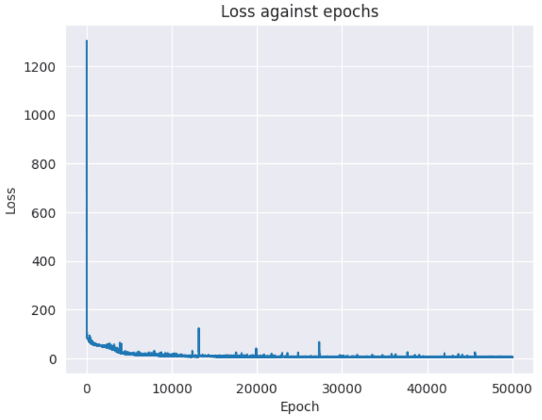
The model is trained for 50000 epochs. You can play around with the number of epochs.
criterion = nn.MSELoss()
optimizer = optim.Adam(model.parameters(), lr=0.001)

num_epochs = 50000

loss_vals = []

for epoch in range(num_epochs):

    optimizer.zero_grad()

    outputs = model(X_train)

    loss = criterion(outputs, y_train)

    loss.backward()

    loss_vals.append(loss.detach().numpy().item())

    optimizer.step()

    if (epoch+1) % 100 == 0:
        print(f'Epoch [{epoch+1}/{num_epochs}], Loss: {loss.item():.4f}')
Output:
Epoch [49100/50000], Loss: 4.1370
Epoch [49200/50000], Loss: 4.2163
Epoch [49300/50000], Loss: 4.7193
Epoch [49400/50000], Loss: 4.5936
Epoch [49500/50000], Loss: 4.5145
Epoch [49600/50000], Loss: 4.0297
Epoch [49700/50000], Loss: 4.0411
Epoch [49800/50000], Loss: 4.1275
Epoch [49900/50000], Loss: 3.9339
Epoch [50000/50000], Loss: 4.9075
Once the model is trained, it’s a good idea to examine how loss decreases with the number of epochs. We’ll generate a plot below showing this relationship.
import seaborn as sns
sns.set_style('darkgrid')
import matplotlib.pyplot as plt


indexes = list(range(len(loss_vals)))

sns.lineplot(x = indexes, y = loss_vals)

plt.xlabel('Epoch')
plt.ylabel('Loss')
plt.title('Loss against epochs')


plt.show()
Output:
Making Predictions on the Test Set
Evaluation of a regression model is different from classification as the output of a regression model is a continuous value. Because of that, we can use mean squared error (MSE) or mean absolute error (MAE) as evaluation metrics.
In the following code, we first turn off the gradient calculation for the model using requires_grad_(False) method. Then, we predict the output of the model on the test data and calculate the MAE and MSE using the mean_absolute_error and mean_squared_error functions from Scikit-learn. Finally, we print out the results.
from sklearn.metrics import mean_squared_error, mean_absolute_error
model.requires_grad_(False)


outputs = model(X_test)

mae = mean_absolute_error(y_test, outputs)
mse = mean_squared_error(y_test, outputs)

print(f'Mean absolute error: {mae:.2f}')
print(f'Mean squared error: {mse:.2f}')
Output:
Mean absolute error: 6.84
Mean squared error: 92.71
The result shows that on average, we are only off by a value of 6.84 for price per unit area of the house. Impressive?
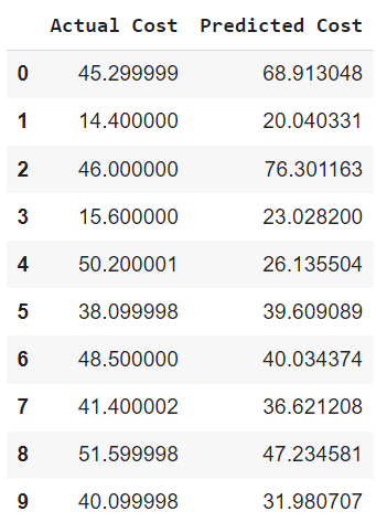
After obtaining the model predictions on the test data, we want to compare the actual and predicted values. To do this, we first need to convert the outputs tensor and the y_test tensor from PyTorch tensors to Python lists.
The outputs.tolist() and y_test.tolist() functions convert the tensors into nested lists, where each sub-list represents a row of data. We then use list comprehension to flatten these lists into a 1-dimensional list, containing all the predictions and actual values.
Finally, we create a pandas DataFrame called results to display the actual and predicted costs of the first 10 houses in the test set. This DataFrame allows us to visually compare the actual and predicted costs of the houses in the test set, which can give us an idea of how well our model is performing.
predictions = [item for sublist in outputs.tolist() for item in sublist]
y_test = [item for sublist in y_test.tolist() for item in sublist]

results = pd.DataFrame({'Actual Cost': y_test, 'Predicted Cost': predictions})
results.head(10)
Output:
Conclusion
In this article, we learned how to use PyTorch to solve both classification and regression problems. We saw how to build a neural network, define the loss function, and optimize the model using both the Adam and SGD optimizers. In classification, we used the cross-entropy loss, while in regression, we used the mean squared error loss. We also saw how to evaluate the model’s performance using various metrics such as accuracy score, mean absolute error, and mean squared error. By using the knowledge gained in this article, you can now apply PyTorch to your own classification and regression projects.
