Time Series Prediction with Hugging Face Transformers

Time series data refers to data dependent on time, such as stock market prices, inflation rates, and daily weather. In some cases, predicting future time series values is crucial. The act of making these predictions is known as time series forecasting or time series prediction.

This tutorial will show you how to classify future time series data using a transformer model from the Python Hugging Face library. Transformer models were initially designed for text-processing tasks such as generation and classification. However, due to the similarity between textual data and time series data in their sequential nature, transformer models have also been adapted for time series data classification.

In this tutorial, we will use the Amazon Chronos transformer from the Hugging Face library to predict future stock prices.

Installing and Importing Required Libraries

The following script downloads the Chronos models.

!pip install git+https://github.com/amazon-science/chronos-forecasting.git

If you’re following this tutorial in Google Colab, you won’t have to install any other libraries.

The script below imports the required libraries into your Python application.

import matplotlib.pyplot as plt
import numpy as np
import pandas as pd
import torch
from sklearn.metrics import mean_absolute_error, mean_squared_error
from chronos import ChronosPipeline

Importing and Preprocessing Stock Market Data

We will use Apple stock price data for the last year (from August 2023 to August 2024) to predict stock prices. We will predict the opening stock price for the last 22 days. This will be our test set. The stock prices for the previous days will be used as the context.

You can download the data from Yahoo Finance in CSV format, or you can copy and paste the history table into an Excel sheet and save it as a CSV - just remember to delete any dividend rows. The script below imports the CSV file into a Pandas DataFrame and displays the data shape and header.

##dataset link
##https://finance.yahoo.com/quote/AAPL/history/

apple_dataset = pd.read_csv("AAPL.csv")
print(apple_dataset.shape)
apple_dataset.head()

Output:

The dataset consists of 252 records. We will predict the opening stock prices using the Chronos model.

As discussed, we will use the last 22 days of data for testing and the remaining data as the context for the time series model. Based on the context, the model will predict the opening stock prices for the last 22 days.

The following script divides the data into test and context sets:

#Calculate the index to split the data
test_size = 22
split_index = len(apple_dataset) - test_size

#If the dataframe is shorter than 22 rows, all goes to test
if split_index < 0:
    train_open = pd.Series(dtype=float)
    test_open = apple_dataset['Open']
else:
    # Splitting the Open column into training and test sets
    train_open = apple_dataset['Open'].iloc[:split_index]
    test_open = apple_dataset['Open'].iloc[split_index:]

Get Our Python Developer Kit for Free

I put together a Python Developer Kit with over 100 pre-built Python scripts covering data structures, Pandas, NumPy, Seaborn, machine learning, file processing, web scraping and a whole lot more - and I want you to have it for free. Enter your email address below and I'll send a copy your way.

Importing Chronos Time Series Model Making Predictions using

We will create a Hugging Face pipeline that uses the amazon chronos-t5-tiny model for time series prediction. You can also use the mini, small, base, or large models.

pipeline = ChronosPipeline.from_pretrained(
  "amazon/chronos-t5-tiny",
  device_map="cuda",
  torch_dtype=torch.bfloat16,
)

Next, we’ll convert the context or training data to PyTorch tensors since the Chronos models use PyTorch on the backend.

Finally, you need to pass the context and the prediction length (22 in this case) to the pipeline’s predict() method to make predictions.

context = torch.tensor(train_open)
prediction_length = test_size
forecast = pipeline.predict(context, prediction_length)

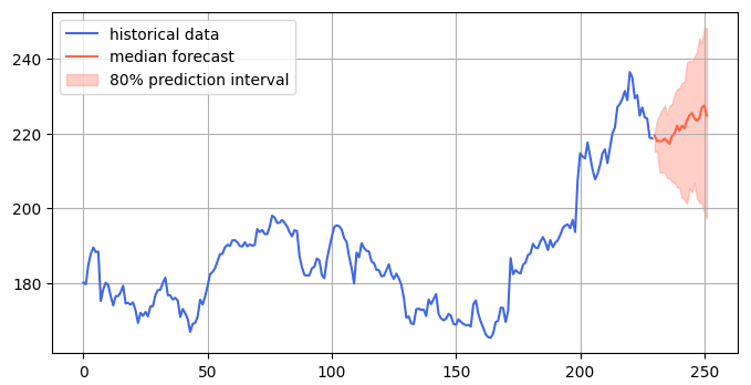
The Chronos models make 20 predictions for each time step. We will divide the data into ten quartiles and take the prediction for the 1st, 5th, and 9th quartiles. The 5th quartile represents median values. The data between the 1st and 9th quartiles will represent the 80% prediction interval.

Next, we can plot the context and the median predictions in a single figure, as shown in the following script:

forecast_index = range(len(train_open), len(train_open) + prediction_length)
low, median, high = np.quantile(forecast[0].numpy(), [0.1, 0.5, 0.9], axis=0)

plt.figure(figsize=(8, 4))
plt.plot(train_open, color="royalblue", label="historical data")
plt.plot(forecast_index, median, color="tomato", label="median forecast")
plt.fill_between(forecast_index, low, high, color="tomato", alpha=0.3, label="80% prediction interval")
plt.legend()
plt.grid()
plt.show()

Output:

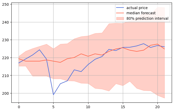
Finally, we will plot the predicted and actual stock prices in the test set in a single plot.

forecast = np.squeeze(forecast)  
low, median, high = np.quantile(forecast, [0.1, 0.5, 0.9], axis=0)
forecast_index = range(len(test_open))

plt.figure(figsize=(8, 5))
plt.plot(forecast_index, test_open, color="royalblue", label="actual price")
plt.plot(forecast_index, median, color="tomato", label="median forecast")
plt.fill_between(forecast_index, low, high, color="tomato", alpha=0.3, label="80% prediction interval")
plt.legend()
plt.grid()
plt.show()

Output:

You can see that most of the predictions are within an 80% prediction interval, with the later predictions being highly accurate.

Let’s calculate the mean absolute error values to see how much the model err on average.

mae = mean_absolute_error(test_open, median)
print("Average open values in the training set:", train_open.mean())
print("Mean Absolute Error (MAE):", mae)

Output:

Average open values in the training set: 186.99199952608697
Mean Absolute Error (MAE): 4.38785126586283

The above output shows that, on average, our model predictions are more than 4 points off, which is 2.1% of the average stock prices in the training set. This is impressive, given that the model is not trained on any data but uses context and the pre-trained weights to predict future time series values.

Conclusion

Transformer models have demonstrated state-of-the-art performance for text classification. They have also been developed for time series data prediction.

In this tutorial, you saw how to make time-series predictions for stock market data using Amazon Chronos models from Hugging Face. Though it’d be naive to think this result could be replicated to reliably predict actual stock prices, it’s still a neat demonstration. I encourage you to try this model for other time series tasks. Happy Coding!

P.S. I ran this same experiment with 1-year of VTIAX, and the actual price was consistently outside the 80% prediction interval, so don’t get too excited!

Get Our Python Developer Kit for Free

I put together a Python Developer Kit with over 100 pre-built Python scripts covering data structures, Pandas, NumPy, Seaborn, machine learning, file processing, web scraping and a whole lot more - and I want you to have it for free. Enter your email address below and I'll send a copy your way.