In this tutorial, we’ll explore callback functions in TensorFlow Keras and how they can be used to improve the performance of deep learning models. Callback functions are a powerful tool in Keras that allow you to customize the behavior of the training process by performing certain actions at various points during training.
In this tutorial, we’ll focus on two common use cases for callback functions: early stopping and model saving. We’ll demonstrate how to use early stopping to prevent overfitting and how to save the best model weights based on validation accuracy. By the end of this tutorial, you’ll have a good understanding of how to use callback functions in TensorFlow Keras to improve the performance of your models.
What are callback functions in TensorFlow Keras
Callback functions in TensorFlow Keras are functions that can be executed at certain points during the training process of a deep learning model. Callbacks can be used to monitor and modify the behavior of the training process, such as saving the best model, stopping the training early to avoid overfitting and more.
During the training process, TensorFlow Keras invokes a series of functions that execute at different points in time. For instance, Keras will invoke the on_batch_begin(), on_batch_end(), on_epoch_begin(), and on_epoch_end() functions at different points during the training. With callback functions, you can define functions and specify when to execute them, and what those functions should do.
In Keras, callbacks are passed to the fit() method of the model as a list, during the model training. Once the fit() method is called, the callbacks are executed at specific intervals during training.
Now that we understand what callback functions are in TensorFlow Keras, let’s move on to the next section and discuss why we need them.
Why you need callback functions
Callback functions are an essential tool for training deep learning models in TensorFlow Keras. Here are a few reasons why you might need to use callback functions during your model training:
- Early stopping: Stop training when a monitored metric stops improving.
- Model checkpointing: Save the best performing model or model at regular intervals during training.
- Learning rate scheduling: Adjust the learning rate over time to improve model performance.
- TensorBoard visualization: Write training logs for visualization in TensorBoard.
- Custom logging: Customize the logging behavior, for example by logging additional metrics or outputting logs in a specific format.
- Data augmentation: Apply data augmentation techniques during training, for example by randomly rotating or cropping images.
- Gradient visualization: Visualize the gradients of the model during training, which can help diagnose issues such as vanishing or exploding gradients.
In the following sections, we’ll provide examples of how to use two common callback functions in TensorFlow Keras: early stopping and model checkpointing. We will demonstrate how these functions can be used to prevent overfitting and save the best model during training.
Early stopping to prevent overfitting during training
Overfitting is a common problem in deep learning where a model is trained too well on the training data and ends up performing poorly on unseen data. Early stopping is a technique used to prevent overfitting during model training. It works by monitoring the performance of the model on a validation set during training, and stopping the training process when the model’s performance on the validation set stops improving.
When applied, early stopping allows the model to train until the optimal point, where the performance on the validation set is maximized. Any further training after this point would result in overfitting. By stopping the training process at the optimal point, the model’s ability to generalize to unseen data is improved.
In this section, we’ll see how to implement early stopping using Keras callback functions. First, we will train a model without early stopping to show you what overfitting looks like. Then, we will train a model with early stopping to see how it helps to prevent overfitting.
We’ll be using the IMDB movie review dataset as an example to show how early stopping can help prevent overfitting during model training. The IMDB dataset is a popular dataset that contains reviews of movies along with their corresponding sentiment, either positive or negative.
The following code imports the necessary Keras modules: Sequential, Embedding, LSTM, and Dense. Then, it loads the IMDB movie review dataset using the imdb.load_data() function. The IMDB dataset comes installed with TensorFlow keras. The argument num_words=5000 specifies that we want to keep only the top 5000 most frequently occurring words in the reviews, which helps to reduce the dimensionality of the input data.
Next, we pad the sequences in both the training and test sets to a maximum length of 100 using pad_sequences(). Padding sequences is necessary because the reviews have varying lengths, and we need to ensure that they are all of the same length for the model to be trained effectively.
Finally, we print the shapes of the training and test sets using the shape attribute to confirm that the sequences have been padded to the correct length.
import tensorflow as tf
from tensorflow.keras.datasets import imdb
from tensorflow.keras.models import Sequential
from tensorflow.keras.layers import Embedding, LSTM, Dense

#Load the IMDB movie review dataset

(x_train, y_train), (x_test, y_test) = imdb.load_data(num_words=5000)

maxlen = 100
x_train = tf.keras.preprocessing.sequence.pad_sequences(x_train, maxlen=maxlen)
x_test = tf.keras.preprocessing.sequence.pad_sequences(x_test, maxlen=maxlen)

print("Train set", x_train.shape)
print("Test set", x_train.shape)
Output:
Train set (25000, 100)
Test set (25000, 100)
Example without early stopping
Let’s first demonstrate how model training without early stopping leads to overfitting.
We’ll use an LSTM (Long Short-Term Memory) model, which is a popular type of recurrent neural network that is particularly suited for the classification of textual data. The LSTM model has been shown to achieve excellent results in various natural language processing tasks such as sentiment analysis.
To create the LSTM model, we will first initialize a Sequential object in Keras and add the layers sequentially. The first layer is the Embedding layer that will convert the integer-encoded vocabulary into dense vectors of fixed size. The output of the Embedding layer will be fed to the LSTM layer which will have 32 units. Finally, we add a Dense layer with a single output unit that uses the sigmoid activation function to output the probability of a review being positive. Here’s the code for creating the Keras LSTM model:
#Define the model architecture

model = Sequential()
model.add(Embedding(input_dim=5000, output_dim=32, input_length=maxlen))
model.add(LSTM(32))
model.add(Dense(1, activation='sigmoid'))
The next step is to compile and train the model.
The compile() method compiles the model. We will compile the model with the adam optimizer and binary_crossentropy loss function, which is a common choice for binary classification problems. We will track accuracy as the performance metric.
After compiling the model, we will train it using the fit() method with x_train and y_train as the training data, epochs=10 for the number of epochs, and batch_size=128 for the batch size. The validation data is set to (x_test, y_test) which will be used to evaluate the model after each epoch. Here is the code for compiling and training the model.
#Compile the model

model.compile(optimizer='adam', loss='binary_crossentropy', metrics=['accuracy'])

#Train the model

history = model.fit(x_train, y_train, epochs=10, batch_size=128, validation_data=(x_test, y_test))
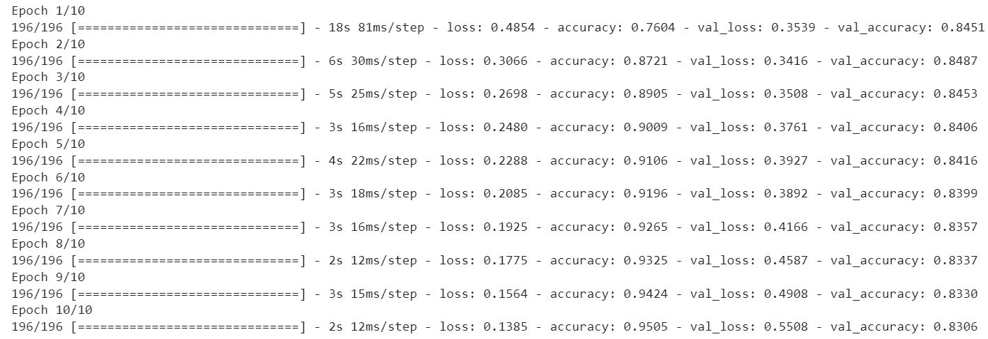
Since we are not using early stopping in this example, the model will train for all 10 epochs, even if it starts to overfit on the training data.
Output:
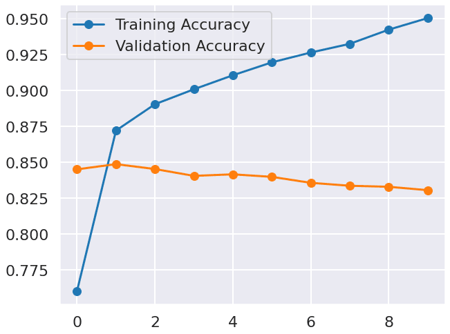
Let’s plot the validation loss and accuracies to see if our model is overfitting.
import matplotlib.pyplot as plt
import seaborn as sns

plt.figure(figsize=(10, 8))
sns.set_style("darkgrid")
sns.set_context("poster")
plt.plot(history.history['accuracy'], label='Training Accuracy', marker='o')
plt.plot(history.history['val_accuracy'], label='Validation Accuracy', marker='o')
plt.legend()
plt.show()
Output:
As we can see from the results, the model achieved the highest accuracy on the validation set (val_accuracy) after the second epoch, with a value of 0.8487. However, after that, the accuracy decreases with each epoch, which suggests that the model is overfitting to the training data. This means that the model is performing well on the training data, but not so well on the validation data or new, unseen data.
Let’s make predictions on the test set.
Note: For demonstration purposes, the test and the validation set used in training are the same in this example.
from sklearn.metrics import accuracy_score

#Make predictions on the test set

y_pred = model.predict(x_test)
y_pred = [1 if p >= 0.5 else 0 for p in y_pred]

#Calculate the accuracy of the predictions

accuracy = accuracy_score(y_test, y_pred)
print("Prediction Accuracy:", accuracy)
Output:
782/782 [==============================] - 3s 3ms/step
Prediction Accuracy: 0.8306
The results above indicate that the model achieved an accuracy of 0.8306 on the test set after the final training. However, during the training process, the model reached its highest accuracy of 0.8487 on the second epoch. These results demonstrate that an overfitted model (trained beyond the second epoch, in this case) tends to perform poorly on the test set.
One way to prevent overfitting is to stop training the model when the performance on the validation set does not improve anymore after a certain number of epochs. This is exactly what early stopping does. It monitors the performance of the model on the validation set during training and stops the training process when the performance does not improve for a certain number of epochs. This way, the model is prevented from overfitting to the training data by stopping the training process before it starts to memorize the training data. In the next section, we’ll show how to implement early stopping in Keras using a callback function.
Example with early stopping
To implement early stopping during training, we can use the EarlyStopping callback from the tensorflow.keras.callbacks module. This callback function monitors a specified metric on a validation set and stops the training process if the metric does not improve for a certain number of epochs.
The EarlyStopping callback takes two main arguments: monitor and patience. The monitor argument specifies the metric that we want to monitor for early stopping. The patience argument specifies the number of epochs to wait before stopping the training process.
Here’s an example of how to define the EarlyStopping callback in Keras:
from tensorflow.keras.callbacks import EarlyStopping

#Define the early stopping callback

early_stopping = EarlyStopping(monitor='val_accuracy', patience=3)
In the above script, we have defined the EarlyStopping callback to monitor the validation accuracy of the model and to stop the training process if the validation accuracy does not improve for three consecutive epochs.
We can then pass this callback as an argument to the fit() method when training the model, as shown in the following code.
When we pass the callback to the fit() method, it gets called at the end of each epoch during training. The callback checks if the monitored metric (val_accuracy, in this case) has improved. If it hasn’t improved for patience number of epochs, the training is stopped early, which can prevent overfitting.
#Define the model architecture
model = Sequential()
model.add(Embedding(input_dim=5000, output_dim=32, input_length=maxlen))
model.add(LSTM(32))
model.add(Dense(1, activation='sigmoid'))


#Compile the model
model.compile(optimizer='adam', loss='binary_crossentropy', metrics=['accuracy'])

#Train the model with early stopping
history = model.fit(x_train, y_train,
                    epochs=10,
                    batch_size=128,
                    validation_data=(x_test, y_test),
                    callbacks=[early_stopping])
Output:
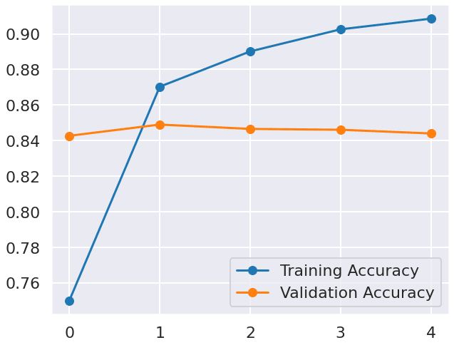
The above results show that the best accuracy on the validation set was achieved after the second epoch, where the validation accuracy was 0.8490. However, after that epoch, the accuracy did not improve for three consecutive epochs, indicating that the model was not improving and may have started to overfit the training data. Since we implement early stopping, the model will not train for 10 epochs but will rather stop at 5 epochs.
Let’s plot the validation accuracy and loss to visually see this training behaviour.
plt.figure(figsize=(10, 8))
sns.set_style("darkgrid")
sns.set_context("poster")
plt.plot(history.history['accuracy'], label='Training Accuracy', marker='o')
plt.plot(history.history['val_accuracy'], label='Validation Accuracy', marker='o')
plt.legend()
plt.show()
Output:
Let’s again make a prediction on the test set.
#Make predictions on the test set
y_pred = model.predict(x_test)
y_pred = [1 if p >= 0.5 else 0 for p in y_pred]

#Calculate the accuracy of the predictions
accuracy = accuracy_score(y_test, y_pred)
print("Prediction Accuracy:", accuracy)
Output:
782/782 [==============================] - 3s 3ms/step
Prediction Accuracy: 0.844
The above result show that we achieve a better accuracy (0.844) than what we got without early stopping (0.8306). However, this accuracy is still less than the best case accuracy of 0.8490 achieved after the second epoch.
The reason behind this behaviour is that, though we implemented early stopping to stop training the model if the validation accuracy doesn’t improve for three consecutive epochs, our model still overfitted for at least three epochs. What we really want is the best model, i.e. the model trained after the second epoch. One way to get the best model is to save the model whenever we achieve the best validation accuracy. After the training we retrieve the saved model (which had the best accuracy on the validation set), and use it to make predictions on the test set. This is what we’ll teach you how to do in the next section.
Saving the best model using callback functions
The ModelCheckpoint callback is used to save the model during training in Keras. This callback can be used in conjunction with early stopping to save the best model that achieved the highest accuracy on the validation set.
For example, the following code above defines two callbacks. The first callback is early_stopping, which we have already discussed. The second callback is checkpoint, which is used to save the best model during training.
The ModelCheckpoint callback takes several arguments. The first argument is the name of the file where the best model will be saved. In this case, the name of the file is monitor, specifies the metric to monitor during training. In this case, we monitor val_accuracy.
The mode argument specifies whether we want to maximize or minimize the monitored metric. Since we want to maximize the accuracy, we set the mode to max. The save_best_only argument specifies whether to save only the best model during training. If set to True, only the best model will be saved.
from keras.callbacks import ModelCheckpoint, EarlyStopping

#Define the callbacks
early_stopping = EarlyStopping(monitor='val_accuracy', patience=3)
checkpoint = ModelCheckpoint('best_model.h5',
                             monitor='val_accuracy',
                             mode='max',
                             save_best_only=True, verbose=1)
In order to use the EarlyStopping and ModelCheckpoint callbacks during training, both callbacks need to be passed in a list to the callbacks argument of the fit() method.
#Define the model architecture
model = Sequential()
model.add(Embedding(input_dim=5000, output_dim=32, input_length=maxlen))
model.add(LSTM(32))
model.add(Dense(1, activation='sigmoid'))

#Compile the model
model.compile(optimizer='adam', loss='binary_crossentropy', metrics=['accuracy'])

#Train the model with early stopping and model saving

history = model.fit(x_train, y_train,
                    epochs=10,
                    batch_size=128,
                    validation_data=(x_test, y_test),
                    callbacks=[early_stopping, checkpoint])
Output:
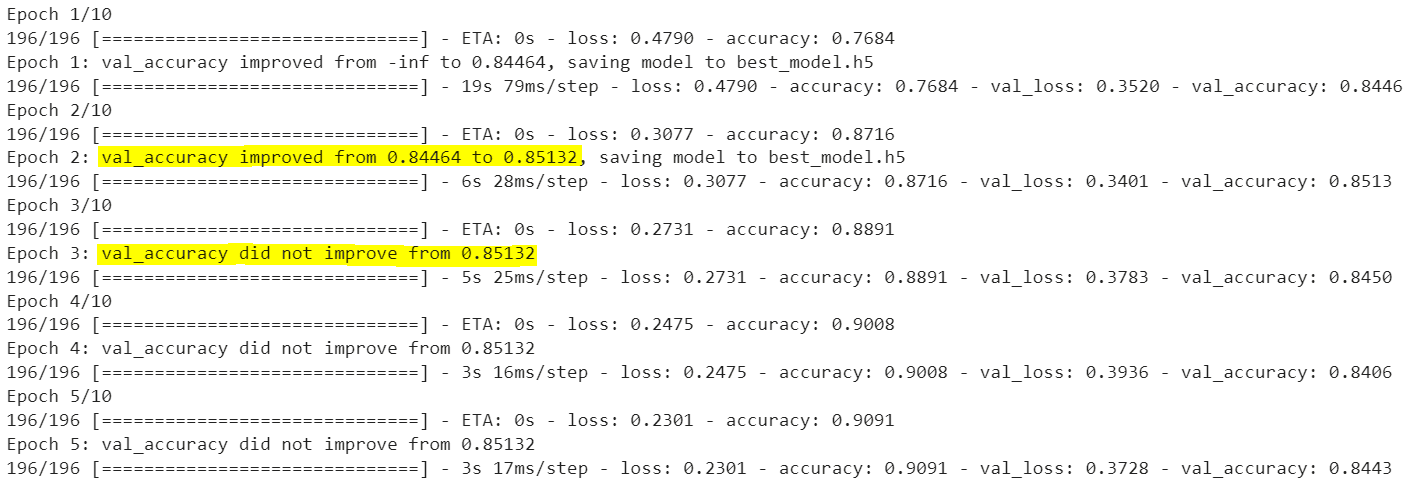
The above output shows that the ModelCheckpoint callback is working as expected. During the training, after each epoch, the callback checks if the val_accuracy has improved or not. If the val_accuracy has improved, then it prints a message stating the val_accuracy has improved and saves the model to the file val_accuracy, so far. If the val_accuracy does not improve, then the callback does not save the model, as we can see in the output.
Let’s print validation loss and accuracies.
plt.figure(figsize=(10, 8))
sns.set_style("darkgrid")
sns.set_context("poster")
plt.plot(history.history['accuracy'], label='Training Accuracy', marker='o')
plt.plot(history.history['val_accuracy'], label='Validation Accuracy', marker='o')
plt.legend()
plt.show()
Output:
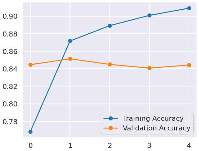
The output again shows that the best validation accuracy is achieved after second epoch. So the best saved model is the one trained after the second epoch.
Let’s first make predictions on the test using the model trained on all five epochs.
#Make predictions on the test set
y_pred = model.predict(x_test)
y_pred = [1 if p >= 0.5 else 0 for p in y_pred]

#Calculate the accuracy of the predictions
accuracy = accuracy_score(y_test, y_pred)
print("Prediction Accuracy:", accuracy)
Output:
782/782 [==============================] - 3s 3ms/step
Prediction Accuracy: 0.84428
The model achieves an accuracy of 0.84428 which is less than the best case accuracy of 0.85132.
Let’s now make predictions on the test set using the best saved model. You can load the best saved model using the load_model() function, like we do in this example:
from keras.models import load_model

#Load the best model
best_model = load_model('best_model.h5')

#Make predictions on the test set
y_pred = best_model.predict(x_test)

y_pred = [1 if p >= 0.5 else 0 for p in y_pred]

#Calculate the accuracy of the predictions
accuracy = accuracy_score(y_test, y_pred)
print("Prediction Accuracy:", accuracy)
Output:
782/782 [==============================] - 3s 3ms/step
Prediction Accuracy: 0.85132
Voila! You can see that now our model achieves the best case accuracy of 0.85132.
In conclusion, the EarlyStopping and ModelCheckpoint callbacks are powerful tools in Keras to prevent overfitting and achieve better model performance. By using these callbacks in conjunction, you can save the best model during training and stop training when the performance on the validation set no longer improves. This approach saves computation time and resources while ensuring that the model generalizes well to unseen data.
For more Python and machine learning tips, subscribe using the form below.
