VBA Transpose to switch rows and columns

Use VBA transpose to switch rows and columns in Excel. The VBA transpose function is helpful for converting rows to columns and columns to rows. In this tutorial, a macro that transposes both data and formatting is presented.

You’re probably familiar with the term “transpose,” which means to “exchange places with” or “transfer to a different place or context,” but what exactly does transpose mean in a VBA context and which Excel objects can we transpose?

To answer these questions, let’s start by giving the formal algebraic definition of transpose as it applies perfectly to the topic of this tutorial. According to English Wikipedia, “…the transpose of a matrix is an operator which flips a matrix over its diagonal, that is it switches the row and column indices of the matrix by producing another matrix…”. In other words, a transposed matrix is a matrix obtained from a given matrix by interchanging each row and its corresponding column.

An Excel worksheet is nothing more than a large matrix consisting of rows and columns. By transposing a subset of a worksheet area, i.e. a data matrix within it, the rows and columns of the data matrix switch places.

Akin to the mathematical definition of a matrix, we may define a data matrix as a collection of data arranged into a fixed number of rows and columns in a range of an Excel worksheet. That is, a data range must have at least two adjacent rows and columns of data to qualify as a data matrix, which explains why we didn’t simply use the term “data range” instead of “data matrix”.

Note, however, that the term data matrix does not refer to a table (a VBA list object) in this context. We need to make this distinction since a table or list object cannot be transposed without being transformed to a non-list object, like a regular data matrix! You can manually create a table or list object in your worksheet in the Insert menu by clicking “Table”, whereas all you need to do to create a data matrix is to put data in some adjacent rows and columns of your worksheet. More on this later.

In an Excel VBA context, transpose is primarily used in conjunction with range objects for presenting data differently, and we’ll focus exclusively on that type of use in this tutorial.

First, we’ll show you a VBA procedure which transposes a matrix, cell by cell, just to give you a clearer picture of how this operation works. Next, we’ll show you a much simpler procedure which utilizes the built-in VBA transpose method to get the same result. However, as will become clear, both procedures are only suitable if you don’t need your existing formatting to be transposed as well. To address this shortcoming, we’ll finish with a more sophisticated VBA macro which allows you to transpose both the data matrix and its formatting. We’ll end the tutorial by discussing some application ideas and situations where you’re better off not transposing your data matrix.

After this somewhat lengthy and technical introduction, let’s get started with our VBA transpose examples!

Macro to transpose cell by cell

Start by adding a new sheet to your workbook and copy-paste the data below into cell “A1” of the empty sheet:

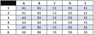
Now add a background color to every other row of the sheet and make the headers bold so that your data matrix looks something like this:

VBA Transpose example data

Next, paste the code below into a standard code module. Caution:  The procedure above will remove the formatting, so before you move on, be sure to make a copy of the formatted data matrix you’ve just created before you run the procedure. You’ll need it later in this tutorial!

Sub InvokeTransposeMatrixCellByCellClearFormatting()
    Call TransposeTableCellByCellClearFormatting (Range("A1").CurrentRegion)

End Sub

Sub TransposeMatrixCellByCellClearFormatting(rng As Range)
    ' (1) copy values in table
    ' (2) clear table and formatting
    ' (3) transpose table cell by cell
    
    Dim lngCol As Long, lngRow As Long
    Dim varArray As Variant
    

    Application.ScreenUpdating = False
    
    With rng
        
        ' (1) copy values in table
        varArray = .Value
        
        ' (2) clear table
        .Clear
        
        ' (3) transpose table cell by cell
        For lngCol = 1 To UBound(varArray)
            For lngRow = 1 To UBound(varArray, 2)
                .Cells(lngRow, lngCol) = varArray(lngCol, lngRow)
            Next lngRow
        Next lngCol
        
    End With
    
    Application.ScreenUpdating = True

End Sub

Make powerful macros with our free VBA Developer Kit

Tutorials like this can be complicated. That’s why we created our free VBA Developer Kit and our Big Book of Excel VBA Macros to supplement this tutorial. Grab them below and you’ll be writing powerful macros in no time.

Use the InvokeTransposeTableCellByCellClearFormatting procedure to call the TransposeTableCellByCellClearFormatting procedure. Okay, yeah I got a little carried away with the macro names!

Both procedures accept only one parameter, the range of your data matrix. This range is then passed from the former procedure to the latter. However, in the former procedure we’ve specified the range by means of the .CurrentRegion range property. This property will determine the range of the entire data matrix based on only one of the contained cells within it, in this case cell “A1”. We use this property because it’s a quick and fairly reliable way to work with a data matrix if you don’t know the exact range. Just make sure your data range qualifies as a data matrix, like we defined in the introduction!

The TransposeTableCellByCellClearFormatting procedure copies the values of the passed range into an array and then clears the original matrix. We do the latter because the example matrix is rectangular rather than quadratic and thus changes shape after being transposed. In other words, since we’re inserting the transposed matrix from the same starting range address (“A1”) as the old matrix, there would be remnants of the original matrix if we didn’t first clear it on our spreadsheet.

Since we’re copying the value of a range, the array Excel returns is two-dimensional. We have to loop through both dimensions of the array in a double or “nested” loop. UBound(varArray) is the number of rows in the passed range and UBound(varArray, 2) is the number of columns. Our UBound tutorial talks more about looping through VBA arrays.

In the inner loop, we then switch the row index with the column index and insert the inverted value cell by cell. That’s all there is to it!

However, this approach has several shortcomings. First of all, accessing and writing to the document is an expensive operation (in terms of time and memory) and doing this cell by cell can be horribly slow, especially if your data matrix is large. In other words, this procedure is not very efficient. Secondly, you lose any formatting of the data. That likely isn’t your desired outcome.

Let’s end this section on that sad note and instead look at the built-in transpose method which fixes these problems!

VBA WorksheetFunction.Transpose

Paste this much shorter code below into a standard code module:

Sub InvokeTransposeMatrixAndKeepFormatting()
    Call TransposeMatrixAndKeepFormatting(Range("A1").CurrentRegion)
End Sub

' Note, this procedure is only suitable for (formatted) quadratic matrices,
' i.e. matrices with an equal number of rows and columns
Sub TransposeMatrixAndKeepFormatting(rng As Range)
    With rng
        .Cells(1, 1).Resize(.Columns.Count, .Rows.Count) = _
            WorksheetFunction.Transpose(.Value)
    End With
End Sub

Next, make another copy of the example data matrix from earlier in this tutorial and paste it in into cell “A1” of an empty worksheet. Now run the InvokeTransposeMatrixAndKeepFormatting procedure and what you’ll see is something like this:

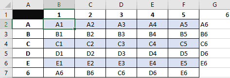
VBA WorkSheetFunction.Transpose data matrix

At a first glance, it looks like the procedure has failed, when in fact it hasn’t! Recall that the example data matrix from is rectangular because it has one more row than columns. Since this procedure doesn’t clear the data matrix range before transposing it, there are bound to be remnants or “leftovers” from the original data matrix because the transposed data matrix doesn’t cover it perfectly. The remnants are in this case the cells in row 7 in the picture above. Moreover, since WorksheetFunction.Transpose doesn’t alter the formatting of the processed range, column G in the picture above is left unformatted as column G wasn’t part of the original data matrix.

This shows us that WorksheetFunction.Transpose works just like the procedure in the previous section, except that it keeps the formatting of the data matrix. In fact, if you comment out the .Clear method in the TransposeMatrixCellByCellClearFormatting procedure, the two procedures become functionally equivalent, except for special cases. We’ll explain what these are later.

The crucial difference between the two procedures is the left-hand side of the statement inside the With rng clause, i.e.:

.Cells(1, 1).Resize(.Columns.Count, .Rows.Count)

Before we can insert the transposed data back into the worksheet, we must specify exactly which range it will occupy. We start out in the top left corner of the input range with .Cells(1, 1) and then resize the output range with the .Resize method of the range object. This method takes two parameters, the number of rows and columns of the resized range. To obtain the correct resizing we simply pass the number of columns and rows of the input range and switch their positions. In other words, in a “normal” .Resize statement, the code would have looked something like this: .Resize(.Rows.Count, .Columns.Count), but since the data is now transposed we need to switch the parameters in case the shape of the input range isn’t quadratic.

In short, this approach allows us to pass both quadratic and rectangular shaped data matrices as input ranges to the procedure.

Even though we’ve made some improvement compared to the first procedure, it still has several shortcomings. First of all, you need to remove the remnants of the original data matrix either manually or by adding additional code. Secondly, if the transposed data matrix is of a different shape than the original, you also have to add some formatting to the output range. Thirdly, if you also want to transpose the formatting of the input range, you still have most of your work ahead of you. That is, if you stick to this approach.

The WorksheetFunction.Transpose method also has a less obvious limitation, albeit a really important one. It won’t work properly if you’re trying to transpose more than 65536 rows (the number of rows in Excel 97-2003).

Let’s look at the third and final approach which takes care of all the shortcomings mentioned above.

VBA to Tranpose both data and formatting

For the grand finale, paste the code below into a standard code module:

Sub InvokeTransposeMatrixAndFormatting()
    Call TransposeMatrixAndFormatting(Range("A1").CurrentRegion)
End Sub

Sub TransposeMatrixAndFormatting(rng As Range)
    ' (1) exit sub if passed range is a table
    ' (2) add new sheet to workbook
    ' (3) disable autofilters, if any
    ' (4) create transposed table in temp sheet
    ' (5) clear current table, copy table from temp sheet and
    '     insert in original sheet
    ' (6) reapply autofilters, if any
    ' (7) clean up: delete new sheet without prompt
    

    Dim blAutoFilter As Boolean
    Dim rngNew As Range
    Dim strRngAddress As String, strTableName As String
    Dim shtNew As Worksheet
    
    Application.ScreenUpdating = False
    
    With rng
    
        .Select
    
        ' (1) exit sub if passed range is a table
        On Error Resume Next
        strTableName = .ListObject.Name
        If strTableName <> vbNullString Then
            MsgBox "The passed range is a table (list object) and cannot be transposed!", _
                vbExclamation, "Error!"
            Exit Sub
        End If
        On Error GoTo 0
        
        strRngAddress = .Address
        
        ' (2) add new sheet to workbook
        Set shtNew = ThisWorkbook.Sheets.Add
    
        ' (3) disable autofilters, if any
        If .Worksheet.AutoFilterMode Then
            blAutoFilter = True
            .Worksheet.AutoFilter.ShowAllData
        End If
    
        .Copy
        
        ' (4) create transposed table in temp sheet
        With shtNew
            Set rngNew = .Range(strRngAddress)
            rngNew.PasteSpecial Paste:=xlPasteAll, Transpose:=True
        End With
        
        ' (5) clear current table, copy table from temp sheet and
        '     insert in original sheet
        .Clear
        rngNew.CurrentRegion.Copy Destination:=rng
        
        ' (6) reapply autofilters, if any
        If blAutoFilter Then .AutoFilter
        
    End With
    
    ' (7) clean up: delete new sheet without prompt
    With Application
        .DisplayAlerts = False
        shtNew.Delete
        .DisplayAlerts = True
        .ScreenUpdating = True
    End With

End Sub

Make another copy of the example data matrix from earlier in this tutorial and paste it in into cell “A1” of an empty worksheet. Now run the InvokeTransposeMatrixAndFormatting procedure and what you’ll see is a new matrix like this:

VBA Transposed Data and Formatting

Voila! Our input data matrix and its formatting has been transposed! Let’s step through the procedure and explain how we achieved this.

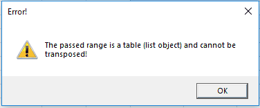
In the first section of the procedure, we introduced a safeguard against passed ranges that are tables (list objects). In case you pass an input data range which is a table, the procedure will terminate with the following error message:

VBA Input data matrix is table error

We check whether the input range is a table by attempting to obtain the name of the list object (table) pertaining to the passed input range in the following conditional statement: If .ListObject.Name <> vbNullString Then. We wrap this condition in On Error Resume Next and On Error Goto 0 to suppress interruption of code execution, since the statement will otherwise cause a run-time error whenever the passed input range is not a table. (We’ll explain in a moment why tables aren’t allowed as input data ranges in this procedure).

Next, we add a temporary blank new sheet to the workbook, which we’ll later use for operations on the passed input range. We also detect whether the passed input range has any active autofilters in the header row with the purpose of later applying the same setting to the transposed data matrix.

The heart of the procedure is this line of code:

rngNew.PasteSpecial Paste:=xlPasteAll, Transpose:=True

Here we paste the input range into the new sheet using .PasteSpecial and the transpose parameter set to True. We need to do this before we clear the input range as the .Clear command in the next line of code empties the content of the Clipboard! To learn more, we’ve created a nice tutorial about some of the other neat things you can do with VBA PasteSpecial.

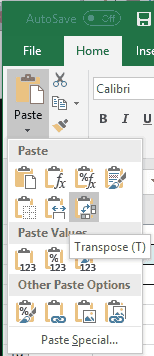
But back to why we don’t allow tables (list objects) to be passed in the parameter to the procedure. Normally, when you copy a range of cells to the clipboard you can then click Home > Paste and choose paste-transpose:

Paste options transpose

However, in case you’ve copied a table to the clipboard, the paste-transpose option is removed from the dropdown options. Excel simply doesn’t allow this for paste jobs and therefore we can’t allow it either when we’re using VBA to paste data into a range.

After transposing the input data range, we simply clear the original range, copy the new data matrix to the original range, reapply the autofilters on the range object and delete the temporary sheet!

Normally, when you delete a worksheet you’ll be prompted with a Yes/No dialog box asking you to confirm the deletion, but we use .DisplayAlerts = False to suppress this dialog box so the procedure can execute smoothly without unnecessary interruptions.

VBA Transpose Application Ideas

We ended up with a relatively sophisticated procedure which transposes both data and formatting in the input data range, but even this procedure has its limitations. Here are a few of them:

• Transpose data matrix to another output range. Throughout this tutorial we’ve been transposing data matrices back to their original ranges, but you could also create transposed copies of your data matrices and place them in new ranges instead. All it takes is that you specify another output range in your procedure. All other things equal, this is a safer course of action, particularly if you’re worried that you might otherwise make unrecoverable mistakes in your data set.
• Do NOT transpose your data matrix if it contains formulas. Your formulas will be transformed into values when transposed and if you overwrite the original data matrix with the transposed data matrix your formulas will be lost unless you close down the workbook without saving your changes!
• Be careful transposing tables (list objects). Tables (list objects) can be transposed with the first or second procedure in this tutorial. However, if you choose to do so, your tables will either be transformed to regular data matrices or left malformed in the process due to the limitations of these procedures. This is probably not the result you want and for this reason we’ve avoided transposing any tables throughout this tutorial.

Finally, it should be noted that the three different procedures presented in this tutorial produce very different results if you pass an input range to them with only one column or one row. They’ll all still work, but we’ll leave it up to you to play around with them and discover exactly how they differ in this respect. You might be surprised by the results!

That’s all for this tutorial. When you’re ready to take your VBA to the next level, subscribe using the form below.