How Feature Scaling Improves Model Training in Deep Learning

Do you know what feature scaling is? We’re going to explain that and show you how it can improve the performance of your deep learning model. With a practical example, we’ll explain the process of feature scaling in TensorFlow Keras. You’ll see that a model trained using scaled features converges faster and is often more accurate, even when trained using a smaller number of epochs.

What is Feature Scaling?

Feature scaling is a technique to standardize the independent features present in the data in a fixed range. Feature scaling is performed during the data preprocessing step to handle features with varying magnitudes, values, or units.

Without feature scaling, a machine learning algorithm assigns larger weights to higher values and smaller weights to lower values, which may result in slow model convergence and, subsequently, lower model accuracy.

Why Feature Scaling is Useful?

Feature scaling is helpful because:

• it ensures all features are on a comparable scale and have comparable ranges, which reduces the dominance of one feature over the others.
• it improves algorithm performance and convergence speed.
• it prevents numerical instability and overflow or underflow problems, which helps avoid errors or inaccuracies due to extreme values.

Types of Feature Scaling

There are two main types of feature scaling: standardization and normalization.

Standardization

Standardization rescales each feature to have a mean of 0 and a standard deviation of 1. It centers data around the mean and adjusts based on variance without changing the original shape of the distribution.

Normalization

Normalization scales each feature to a specific range, like [0, 1], or to have a unit norm. This process changes the range of the data but preserves its original distribution, ensuring equal contribution of features in analysis.

Both standardization and normalization have advantages and disadvantages depending on the data and model. Some general guidelines are:

• Standardize if your data has outliers or skewed distributions.
• Normalize if your data has different units or scales.
• Use standardization and normalization together if your data has outliers and different units.
• Avoid both standardization and normalization if your data has similar distributions or units.

Get Our Python Developer Kit for Free

I put together a Python Developer Kit with over 100 pre-built Python scripts covering data structures, Pandas, NumPy, Seaborn, machine learning, file processing, web scraping and a whole lot more - and I want you to have it for free. Enter your email address below and I'll send a copy your way.

Feature Scaling Example in TensorFlow Keras

In this section, we will see how feature scaling can improve the performance of a deep learning model with the help of a TensorFlow Keras example.

We will use a customer churn dataset from Kaggle, which contains information about bank customers and whether they exited (or churned). Our goal is to build a binary classifier that can predict whether a customer will exit based on their features. This is similar to what we build years ago when introducing scikit-learn machine learning.

Importing Required Libraries

The following script imports the libraries you will need to run scripts in this tutorial.

import seaborn as sns
sns.set_style(style="darkgrid")

import pandas as pd
pd.set_option('display.float_format', lambda x: '%.3f' % x)

import matplotlib.pyplot as plt

from sklearn.model_selection import train_test_split
from sklearn. preprocessing import StandardScaler
from sklearn. preprocessing import MinMaxScaler

from keras.models import Sequential
from keras.layers import Dense

Importing and Preprocessing the Dataset

The script below imports the dataset CSV file into a Pandas DataFrame and displays its first few rows.

customer_data = pd.read_csv('/content/Churn_Modelling.csv')
print(customer_data.shape)
customer_data.head()

Output:

You can see that the dataset contains a lot of customer information, including geography, age, gender and estimated salary. The Exited column contains information about whether or not a person left the bank.

The RowNumber, CustomerId, and Surname columns in our dataset are not helpful in training a churn prediction model, so we’re going to remove these columns.

customer_data = customer_data.drop(['RowNumber', 'CustomerId', 'Surname'], axis=1)

Next, we will convert all the categorical columns in the dataset to one-hot encoded numerical columns.

categorical_columns = customer_data.select_dtypes(include=['object']).columns
customer_data_encoded = pd.get_dummies(customer_data, columns=categorical_columns, drop_first=True)

The next step is to divide the dataset into a features and labels set.

X = customer_data_encoded.drop('Exited', axis=1)
y = customer_data_encoded['Exited']

Finally, we will divide the dataset into 80% training and 20% test sets.

X_train, X_test, y_train, y_test = train_test_split(X, y, test_size=0.2, random_state=42)

Before we train the model, let’s display the mean and standard deviation values for all the columns in our dataset.

X_train.describe()

Output:

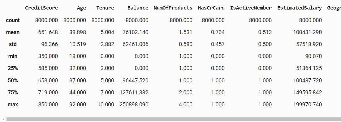
The above output shows that the dataset features have very different magnitudes. For example, the Age column has a mean value of 38.898 while the EstimatedSalary column has a mean value of 100431.290. This vast difference between the values of different features can result in fluctuating training loss and very slow training. Let’s see this with an example.

Model Training without feature scaling

Let’s create a simple Keras sequential model. The model will have two hidden layers with 64 and 32 nodes, respectively.

The output layer will have a single node with a sigmoid activation function since we want to predict a probability value between 0 and 1.

We will use the Adam optimizer and the binary cross entropy loss function since we are solving a binary classification problem.

The fit() method trains the model for 20 epochs using unscaled training and test sets.

model = Sequential()
model.add(Dense(64, activation='relu', input_shape=(X_train.shape[1],)))
model.add(Dense(32, activation='relu'))
model.add(Dense(1, activation='sigmoid'))

model.compile(loss='binary_crossentropy', optimizer='adam', metrics=['accuracy'])

history = model.fit(X_train, y_train, epochs=20, batch_size=32, validation_split=0.2)

Let’s plot the loss across epochs and the model performance on the test set.

plt.plot(history.history['loss'])
plt.plot(history.history['val_loss'])
plt.title('Model Loss')
plt.ylabel('Loss')
plt.xlabel('Epoch')
plt.legend(['Train', 'Validation'], loc='upper left')
plt.show()

loss, accuracy = model.evaluate(X_test, y_test)
print(f'Test Accuracy: {accuracy}')

Output:

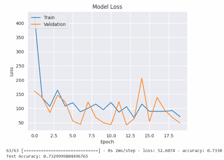
From the above output, you can see that the model cannot converge after 20 epochs, and both training and validation losses keep fluctuating.

You will need a more complex model with more training epochs to achieve convergence. The other option is to use data scaling, as seen in the next section.

Model Training with Feature scaling

This section will show you how to scale training features using standardization and normalization techniques. You will see that the model trained using scaled features will converge very quickly, with model loss consistently decreasing.

Using Standard Scaler

We’re going to use the sklearn. preprocessing.StandardScaler class from the Sklearn library to standardize our data.

To do so, you must create an object of the StandardScaler class and call the fit_transform() method to scale your training data.

Next, you can use the transform() method to scale the test data using the scaling dimensions learned from the training set.

scaler = StandardScaler()
X_train_scaled = scaler.fit_transform(X_train)
X_test_scaled = scaler.transform(X_test)

Now, if you display the mean values of the standardized dataset, you will see them scaled to zero with the standard deviations scaled to one.

X_train_scaled_df = pd.DataFrame(X_train_scaled, columns=X_train.columns)
X_train_scaled_df.describe()

Output:

Next, we will create the same model architecture we did for the unscaled data and train it using the standardized data.

model = Sequential()
model.add(Dense(64, activation='relu', input_shape=(X_train_scaled.shape[1],)))
model.add(Dense(32, activation='relu'))
model.add(Dense(1, activation='sigmoid'))

model.compile(loss='binary_crossentropy', optimizer='adam', metrics=['accuracy'])

history = model.fit(X_train_scaled, y_train, epochs=20, batch_size=32, validation_split=0.2)

The following script plots the model loss across epochs.

plt.plot(history.history['loss'])
plt.plot(history.history['val_loss'])
plt.title('Model Loss')
plt.ylabel('Loss')
plt.xlabel('Epoch')
plt.legend(['Train', 'Validation'], loc='upper left')
plt.show()

loss, accuracy = model.evaluate(X_test_scaled, y_test)
print(f'Test Accuracy: {accuracy}')

Output:

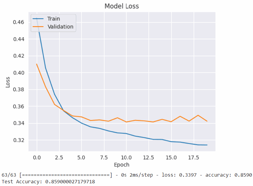
The above output shows that the model converged faster than the unscaled data, and the performance on the test set is much better (85.90%)compared to 73.29% achieved with the unscaled data.

Using normalization

Finally, let’s see an example of data scaling using normalization. To do so, you can use the sklearn. preprocessing.MinMaxScaler class, as the following script demonstrates.

scaler = MinMaxScaler()
X_train_normalized = scaler.fit_transform(X_train)
X_test_normalized = scaler.transform(X_test)

Let’s plot the normalized data to see the difference in the mean values.

X_train_normalized_df = pd.DataFrame(X_train_normalized, columns=X_train.columns)
X_train_normalized_df.describe()

Output:

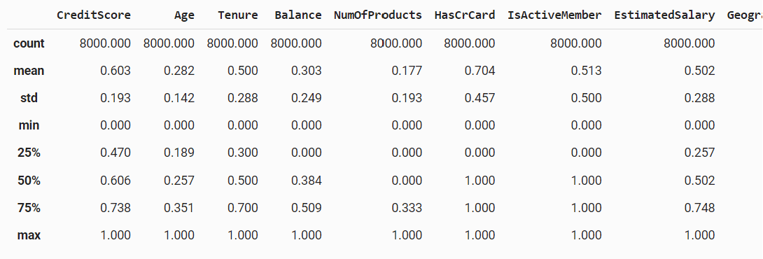
The above output shows that the difference between the magnitude of mean values are not zero but they’re much closer than the unscaled data.

The following script trains our Keras classification model using this normalized data.

model = Sequential()
model.add(Dense(64, activation='relu', input_shape=(X_train_normalized.shape[1],)))
model.add(Dense(32, activation='relu'))
model.add(Dense(1, activation='sigmoid'))

model.compile(loss='binary_crossentropy', optimizer='adam', metrics=['accuracy'])

history = model.fit(X_train_normalized, y_train, epochs=20, batch_size=32, validation_split=0.2)


plt.plot(history.history['loss'])
plt.plot(history.history['val_loss'])
plt.title('Model Loss')
plt.ylabel('Loss')
plt.xlabel('Epoch')
plt.legend(['Train', 'Validation'], loc='upper left')
plt.show()

loss, accuracy = model.evaluate(X_test_normalized, y_test)
print(f'Test Accuracy: {accuracy}')

Output:

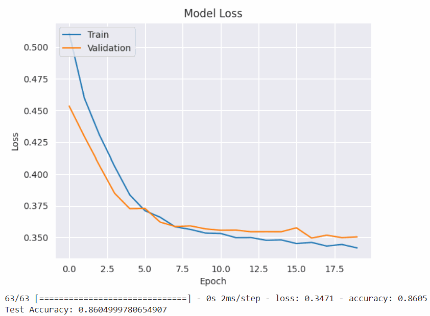
Again, you can see that the model converged faster and achieved much higher accuracy (86.04%) than our original test set.

Conclusion

Data scaling is an important technique to speed up your model convergence and training process. In this tutorial, you saw how to scale your data and achieve model convergence much quicker than with unscaled data.

Both standardization and normalization techniques are used for data scaling. As a rule of thumb, use standardization if your data has outliers or skewed distributions, and use normalization if your data has different units or scales.

For Python tips like this one, go ahead and subscribe using the form below!

Get Our Python Developer Kit for Free

I put together a Python Developer Kit with over 100 pre-built Python scripts covering data structures, Pandas, NumPy, Seaborn, machine learning, file processing, web scraping and a whole lot more - and I want you to have it for free. Enter your email address below and I'll send a copy your way.