Python PCA Examples with sklearn

Principal component analysis, or PCA, is one of the most commonly used dimensionality reduction techniques. Datasets with a large number of attributes, when projected into feature space, can likewise result in a large number of features. This behavior is referred as the “curse of dimensionality,” which can slow down data processing techniques, like when training a machine learning model.

Dimensionality reduction techniques reduce the total number of features in a dataset with minimal affect on the overall data model performance. Another advantage is the reduced feature space allows you to visualize data in two or three-dimensional feature space, whereas that would be near impossible with 8 or 9 features.

PCA is one of the simplest techniques for dimensionality reduction. PCA is an unsupervised dimensionality reduction technique which doesn’t require labeled data. The working principal of PCA is based on the selection of features that cause maximum variance in the overall data distribution. The selected features are called principal components.

The major advantages of PCA are:

1. Fast model training
2. Reduced number of features are easy to visualize
3. Reduced number of features result in less model overfitting.

With the help of an example, we’re going show you how to perform PCA using the Python scikit-learn (sklearn) library. You’ll train a machine learning model on 8 attributes of different patients to solve a binary classification task of predicting whether or not a patient is diabetic. Next, using PCA, you’ll remove some of the features and see if you can still get good prediction performance.

PCA is one technique for dimensionality reduction, but it’s not the only one. If you’d like an alternative, try our tutorial on Python Linear Discriminant Analysis.

Code More, Distract Less: Support Our Ad-Free Site

You might have noticed we removed ads from our site - we hope this enhances your learning experience. To help sustain this, please take a look at our Python Developer Kit and our comprehensive cheat sheets. Each purchase directly supports this site, ensuring we can continue to offer you quality, distraction-free tutorials.

Training a machine learning model with default features

Organizing our data

The dataset we’ll use to train our machine learning model can be downloaded in CSV format from this Kaggle link. It’s been mirrored here in case you prefer to download it directly.

Now that you have the dataset, execute the following script to import our first few required Python libraries:

import pandas as pd
import numpy as np
import seaborn as sns

Our next couple lines of code use Pandas read_csv() to import the dataset we just downloaded. By default, the dataset doesn’t contain any headers so a custom list of headers is defined in our script:

header_list = ["Preg", "Glucose", "BP", "skinThick", "Insulin", "BMI", "DPF", "Age", "Class"]
diabetes_ds = pd.read_csv(r"C:\Datasets\pima-indians-diabetes.csv", names = header_list)

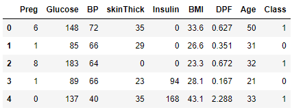
diabetes_ds.head()

The output shows that the dataset contains 9 columns of data. The first 8 columns contain patient attributes on the basis of which the value in the 9th column, Class, will be predicted. Class is simply a binary (0 or 1) result indicating whether or not the patient has diabetes.

Output:

Before you apply any machine learning algorithm to make predictions, you need to divide the dataset into a features and labels set, which is easily done in the following script:

features = diabetes_ds.drop(['Class'], axis=1) #everything but the Class column
labels = diabetes_ds["Class"] #the Class column

The following script divides the dataset into 80% training and 20% test sets using the train_test_split() method from the sklearn.model_selection module. Machine learning models are trained on the training set and evaluated on the test set. The Class of each patient is known in the test set, so that’s how we’re able to evaluate the performance of our trained model.

from sklearn.model_selection import train_test_split

X_train, X_test, y_train, y_test = train_test_split(features, labels,  test_size=0.20, random_state=0)

It’s always a good practice to normalize your data. The following script uses standard scaler to normalize our feature set.

from sklearn.preprocessing import StandardScaler
stand_scal = StandardScaler()
X_train = stand_scal.fit_transform(X_train)
X_test = stand_scal.transform (X_test)

Establish baseline without PCA

Alright, now that we have the data manipulation out of the way, let’s start training our model. For this demonstration, we’re not going to use any dimensionality reduction techniques. That is, we’re not going to use PCA - it’s just going to be a raw machine learning demonstration to establish our baseline algorithm accuracy.

You can use any algorithm to train your machine learning model. For the sake of this example, we’ll use the Random Forest Classifier to train our model. This classifier might sound familiar to you because we used it when we trained our spam email detection model, our Python sentiment analysis demo and several sklearn machine learning examples.

To train with the Random Forest Classifier, you’ll use the fit() method of the RandomForestClassifier class of the sklearn.ensemble module, as shown in the following script. To make predictions on the test set, you need to call the predict() method and pass it your test set.

from sklearn.ensemble import RandomForestClassifier

model = RandomForestClassifier(n_estimators=50, random_state=0)
model.fit(X_train, y_train)
y_pred = model.predict(X_test)

Finally, you can use the accuracy_score() method from the sklearn.metrics module to evaluate the performance of your model.

from sklearn.metrics import accuracy_score
print(accuracy_score(y_test, y_pred))

Output:

0.7987012987012987

The output shows that when using all 8 features, our algorithm achieves an accuracy of 79.87% for correct prediction of whether or not a person is diabetic. That’s not great, but it’s not too bad for a quickly trained model with a limited dataset.

Dimensionality Reduction with PCA

Now that we have our baseline, we’re going to reduce the number of features in our dataset using PCA. We’ll again train our machine learning model on the reduced set of features to see how well our algorithm performs relative to the baseline, unreduced, model we just ran.

To implement principal component analysis with the scikit-learn library, you’ll use the PCA class from the sklearn.decomposition module. The number of desired principal components is passed to the n_components attribute of the PCA class constructor.

Code More, Distract Less: Support Our Ad-Free Site

You might have noticed we removed ads from our site - we hope this enhances your learning experience. To help sustain this, please take a look at our Python Developer Kit and our comprehensive cheat sheets. Each purchase directly supports this site, ensuring we can continue to offer you quality, distraction-free tutorials.

Next, you need to pass your feature set to the fit_transform() method of the PCA class, which returns the data reduced into the specified number of principal components. Since you’ll be evaluating your trained model on the test set, you need to reduce the test set to its principal components, as well. For our test set, you can use the PCA model already trained using the training set, then call the transform method on it and pass it the test set.

The following script reduces the training set into 4 principal components - half the original number of features.

from sklearn.decomposition import PCA

pca_model = PCA(n_components=4)
X_train_pca = pca_model.fit_transform(X_train)
X_test_pca = pca_model.transform(X_test)

Now, let’s again train the Random Forest Classifier algorithm on the reduced feature set and see how well our new model performs.

from sklearn.ensemble import RandomForestClassifier

model = RandomForestClassifier(n_estimators=50, random_state=0)
model.fit(X_train_pca, y_train)
y_pred = model.predict(X_test_pca)

print(accuracy_score(y_test, y_pred))

The output shows that with half number of features, a performance difference of 7% is observed (from 79.87% to 72.72%).

In other words, with 4 principal components, you get an accuracy of around 72% so the extra 4 sets of features only contribute to an increase of around 7% in accuracy.

Output:

0.7272727272727273

This highlights one the key benefits of PCA, or any dimensionality reduction technique. You may sacrifice a little accuracy but you can get a strong performance boost by only evaluating half the number of features.

Let’s now see what our accuracy is like if we only use 2 principal components.

from sklearn.decomposition import PCA

pca_model = PCA(n_components=2)
X_train_pca = pca_model.fit_transform(X_train)
X_test_pca = pca_model.transform(X_test)

from sklearn.ensemble import RandomForestClassifier

model = RandomForestClassifier(n_estimators=50, random_state=0)
model.fit(X_train_pca, y_train)
y_pred = model.predict(X_test_pca)

print(accuracy_score(y_test, y_pred))

The output shows that we get an accuracy of 71.42% using only two principal components out of the original 8 features. This shows that the remaining 6 features only contribute to about an 8.5% increase in accuracy.

Output:

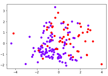
0.7142857142857143

Now that we’ve reduced our dataset into a small number of features, we can actually plot the two principal components and see how our data is distributed based on these two principal components.

from matplotlib import pyplot as plt

plt.scatter(X_test_pca[:,0], X_test_pca[:,1], c= y_test, cmap='rainbow' )
plt.show()

Output:

The choice of the optimal number of principal components depends on your use. It’s always a good idea to start with a small number of principal components and then gradually increase the number until you get your desired results, recognizing that the more principal components you have, the more resource intensive your calculations will be. With that in mind, you can then select the number of principal components after which no significant improvement in model performance is observed.

For more Python machine learning examples, join our mailing list below - we send a new tutorial each week so you can really take your Python programming to the next level.

Code More, Distract Less: Support Our Ad-Free Site

You might have noticed we removed ads from our site - we hope this enhances your learning experience. To help sustain this, please take a look at our Python Developer Kit and our comprehensive cheat sheets. Each purchase directly supports this site, ensuring we can continue to offer you quality, distraction-free tutorials.