Working with TensorFlow Hub Models for Transfer Learning

Transfer learning is a powerful technique in machine learning and deep learning that enables us to leverage knowledge learned from one task and apply it to another related task. It involves using a pre-trained model as a starting point and then fine-tuning it on a new dataset or problem domain. This approach is particularly useful when working with limited data or when training a model from scratch would be computationally expensive and time-consuming.

One of the options for obtaining pre-trained models is through TensorFlow Hub, a repository of pre-trained models and modules for TensorFlow.

In this article, we will explore how to improve the performance of our TensorFlow Keras models using pre-trained models from TensorFlow Hub. We will begin by examining the classification results on the CIFAR dataset using a simple Convolutional Neural Network (CNN) model without transfer learning. The results will demonstrate the limitations of the simple CNN model. However, through the application of transfer learning and incorporating pre-trained models from TensorFlow Hub, we will witness a significant improvement in the model’s performance. So, let’s dive in and discover the power of transfer learning in TensorFlow!

Before we begin, let’s first install the required libraries. You will need to install tensorflow, tensorflow_hub, and keras libraries.

!pip install --upgrade tensorflow tensorflow_hub keras

In addition, for plotting graphs, you will need to install the matplotlib, numpy, and seaborn libraries.

!pip install matplotlib seaborn numpy

The script below imports the libraries you just installed into your Python application:

import tensorflow as tf
import tensorflow_hub as hub
from tensorflow.keras import layers
import numpy as np
import seaborn as sns
import matplotlib.pyplot as plt

Training Keras Model Without Transfer Learning

In this section, we will train a simple Convolutional Neural Network (CNN) model without any transfer learning. We will see what classification results we get without transfer learning, and we’ll later compare these results to the results that we achieve with transfer learning.

As discussed earlier, we will use the CIFAR-10 dataset to train our Keras model in this tutorial. The CIFAR dataset is a collection of labeled images commonly used for computer vision tasks. It stands for the Canadian Institute for Advanced Research, which initiated the dataset’s creation. CIFAR-10, one of its popular variants, consists of 60,000 32x32 color images belonging to 10 different classes, such as airplanes, cars, and cats.

The follow script loads the CIFAR-10 dataset into your Python application, normalizes the image pixel values, and resizes the images to a size of 96x96 pixels.

cifar = tf.keras.datasets.cifar10
(train_images, train_labels), (test_images, test_labels) = cifar.load_data()

train_images = train_images / 255.0
test_images = test_images / 255.0

resized_train_images = tf.image.resize(train_images, (96, 96))
resized_test_images = tf.image.resize(test_images, (96, 96))

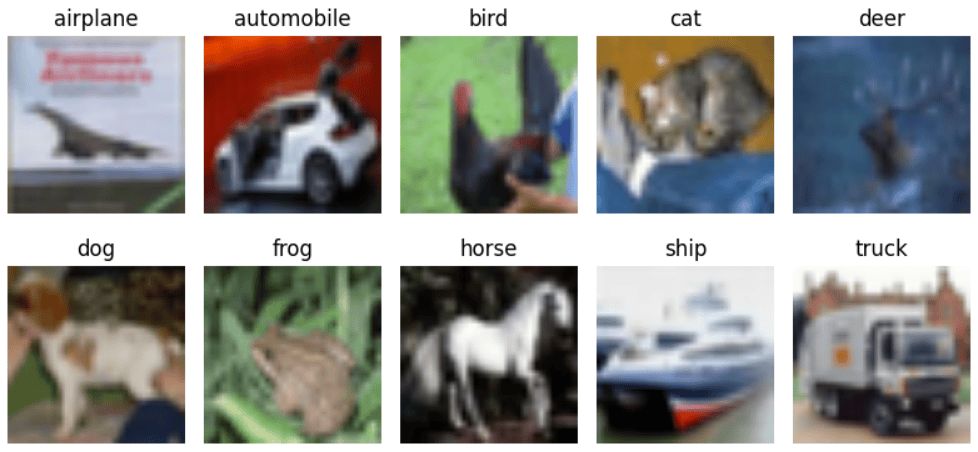
Now, let’s explore the CIFAR-10 dataset by visualizing images from each of its 10 classes.

The following script iterates through the class labels, retrieves the first image for each class from the test images, and plots them with their respective labels using matplotlib. This provides a quick overview of the different classes present in the dataset.

class_labels = ['airplane', 'automobile', 'bird', 'cat', 'deer', 'dog', 'frog', 'horse', 'ship', 'truck']

plt.figure(figsize=(8, 4))
for i in range(10):
    # Find an example image for each class
    class_indices = np.where(test_labels == i)[0]
    image_index = class_indices[0]
    image = resized_test_images[image_index]
    image_label = class_labels[i]

    # Plot image
    plt.subplot(2, 5, i+1)
    plt.imshow(image)
    plt.title(image_label)
    plt.axis('off')

plt.tight_layout()
plt.show()

Output:

Get Our Python Developer Kit for Free

I put together a Python Developer Kit with over 100 pre-built Python scripts covering data structures, Pandas, NumPy, Seaborn, machine learning, file processing, web scraping and a whole lot more - and I want you to have it for free. Enter your email address below and I'll send a copy your way.

Let’s now define a Keras model that doesn’t use any transfer learning for training the model.

As shown in the script below, our model consists of three CNN layers, followed by max pooling layers to extract features from the input images. The flattened output is then passed through dense layers with dropout regularization to reduce overfitting. The model is compiled with the Adam optimizer, sparse categorical cross-entropy loss, and accuracy metric.

#Create the classification model
num_classes = 10  # Number of output classes
model = tf.keras.Sequential([
    tf.keras.layers.Conv2D(32, (3, 3), activation='relu', input_shape=(96, 96, 3)),
    tf.keras.layers.MaxPooling2D((2, 2)),
    tf.keras.layers.Conv2D(64, (3, 3), activation='relu'),
    tf.keras.layers.MaxPooling2D((2, 2)),
    tf.keras.layers.Conv2D(64, (3, 3), activation='relu'),
    tf.keras.layers.Flatten(),
    tf.keras.layers.Dense(256, activation='relu'),
    tf.keras.layers.Dropout(0.5),
    tf.keras.layers.Dense(128, activation='relu'),
    tf.keras.layers.Dropout(0.5),
    tf.keras.layers.Dense(num_classes, activation='softmax')
])

#Compile the model
model.compile(optimizer='adam',
              loss='sparse_categorical_crossentropy',
              metrics=['accuracy'])

Next, we’ll train the model using the fit() function by providing the resized training images and corresponding labels. It is trained for 10 epochs with the validation data being used to monitor the model’s performance during training. After training, the model is evaluated using the resized test images and their labels, and the test loss and accuracy are computed. The model is then used to make predictions on the resized test images using the predict() function.

#Train the model
history = model.fit(resized_train_images,
          train_labels, epochs=10,
          validation_data=(resized_test_images, test_labels)
          )

#Evaluate the model
test_loss, test_acc = model.evaluate(resized_test_images, test_labels)
print(f'Test accuracy: {test_acc}')

#Make predictions
predictions = model.predict(resized_test_images)

Output:

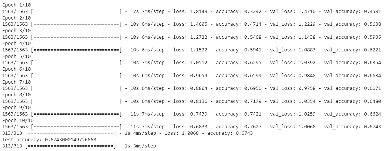
The above output shows that our model achieves a maximum accuracy of 67.43%.

Let’s display our loss and accuracy values across epochs.

sns.set(style="darkgrid")

# Plot loss and accuracy over epochs
plt.figure(figsize=(12, 4))
plt.subplot(1, 2, 1)
plt.plot(history.history['loss'], label='Training Loss')
plt.plot(history.history['val_loss'], label='Validation Loss')
plt.xlabel('Epoch')
plt.ylabel('Loss')
plt.legend()

plt.subplot(1, 2, 2)
plt.plot(history.history['accuracy'], label='Training Accuracy')
plt.plot(history.history['val_accuracy'], label='Validation Accuracy')
plt.xlabel('Epoch')
plt.ylabel('Accuracy')
plt.legend()

plt.tight_layout()
plt.show()

Output:

We can see from the above output that on the test set, our model achieves a validation accuracy of about ~66% around the 6th epoch. For the subsequent epochs, the accuracy fluctuated between 66% and 67%.

In the next section, you will see how transfer learning significantly improves our model performance.

Get Our Python Developer Kit for Free

I put together a Python Developer Kit with over 100 pre-built Python scripts covering data structures, Pandas, NumPy, Seaborn, machine learning, file processing, web scraping and a whole lot more - and I want you to have it for free. Enter your email address below and I'll send a copy your way.

Improving Keras Model Performance Using Transfer learning

For transfer learning, you need a pre-trained model. A pre-trained model is a model that has been trained on a large dataset for a specific task, such as image classification, and has learned useful features and patterns. It allows transfer learning by leveraging the knowledge and representations gained from the pre-training to improve performance on a different but related task.

One of the common sources to obtain pre-trained models is TensorFlow Hub. It offers a wide range of free-to-use models across different domains, allowing users to benefit from transfer learning and leverage the knowledge gained by models trained on large-scale datasets.

To utilize TensorFlow Hub’s pretrained models as Keras layers, you can simply pass the model URL to the hub.KerasLayer class. In the following example, we use the ResNet-50 pretrained model for image classification:

#Load pre-trained ResNet50 model from TensorFlow Hub

model_url = "https://tfhub.dev/google/imagenet/resnet_v2_50/classification/4"
base_model = hub.KerasLayer(model_url, input_shape=(96, 96, 3), trainable=False)

By specifying the model_url and the input shape, the hub.KerasLayer class creates a layer that incorporates the pretrained ResNet-50 model into your architecture. In this case, the model is set to be non-trainable (trainable=False), meaning that the pretrained weights are frozen and won’t be updated during training. If you want to train the ResNet-50 model from scratch, you can set this parameter to true. Just be aware that the model training can take more time.

You can now use the pre-trained ResNet 50 model features in your custom model by incorporating the Keras layer containing the set of ResNet model layers as the base layer in your model. Simply add this layer as the first layer in your model and continue building additional layers on top of it.

The following script demonstrates how to implement this approach, by specifying the <pre>base_model</pre> object we just defined as our first layer.

#Create the classification model
num_classes = 10  # Number of output classes
model = tf.keras.Sequential([
    base_model,
    tf.keras.layers.Dense(256, activation='relu'),
    tf.keras.layers.Dropout(0.2),
    tf.keras.layers.Dense(128, activation='relu'),
    tf.keras.layers.Dropout(0.2),
    tf.keras.layers.Dense(num_classes, activation='softmax')
])

#Compile the model
model.compile(optimizer='adam',
              loss='sparse_categorical_crossentropy',
              metrics=['accuracy'])

The rest of the process is the same as what we did in the first section; you train the model using the fit() method and make predictions using the predict() method.

Let’s run the following script to see if we get better performance with transfer learning.

#Train the model
history = model.fit(resized_train_images,
          train_labels, epochs=10,
          validation_data=(resized_test_images, test_labels)
          )

#Evaluate the model
test_loss, test_acc = model.evaluate(resized_test_images, test_labels)
print(f'Test accuracy: {test_acc}')

#Make predictions
predictions = model.predict(resized_test_images)

Output:

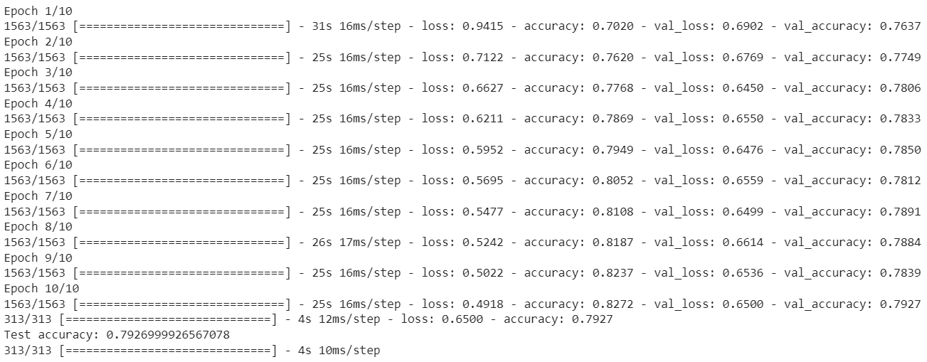
From the output, you can see that even after the first epoch our model achieved an accuracy of 76.37% which is significantly better than the final accuracy (67.43%) achieved by the CNN model after 10 epochs, without transfer learning.

In case of transfer learning, we achieve a performance of 79.26% after 10 epochs.

Let’s plot our new loss and accuracies against epochs.

sns.set(style="darkgrid")

#Plot loss and accuracy over epochs
plt.figure(figsize=(12, 4))
plt.subplot(1, 2, 1)
plt.plot(history.history['loss'], label='Training Loss')
plt.plot(history.history['val_loss'], label='Validation Loss')
plt.xlabel('Epoch')
plt.ylabel('Loss')
plt.legend()

plt.subplot(1, 2, 2)
plt.plot(history.history['accuracy'], label='Training Accuracy')
plt.plot(history.history['val_accuracy'], label='Validation Accuracy')
plt.xlabel('Epoch')
plt.ylabel('Accuracy')
plt.legend()

plt.tight_layout()
plt.show()

Output:

The above output shows that even at initial epochs the performance is much better, and it further improves with each epoch.

In this tutorial, you learned about the power of transfer learning in improving the performance of a Keras model. By leveraging pre-trained models, such as those available in TensorFlow Hub, you can save time and computational resources while achieving better results, especially when working with smaller datasets. Transfer learning is a valuable technique that can significantly enhance the effectiveness of your models, and I encourage you to explore its benefits in your own projects.

Get Our Python Developer Kit for Free

I put together a Python Developer Kit with over 100 pre-built Python scripts covering data structures, Pandas, NumPy, Seaborn, machine learning, file processing, web scraping and a whole lot more - and I want you to have it for free. Enter your email address below and I'll send a copy your way.