Data Scaling and Normalization in Python with Examples

In this tutorial, we’ll study several data scaling and normalization techniques in Python using both sklearn and conventional programming and we’ll share lots of examples. Here are the data scaling techniques we’re going to learn in this tutorial:

1. Standard Scaling
2. Min/Max Scaling
3. Mean Scaling
4. Maximum Absolute Scaling
5. Median and Quantile Scaling

What is Data Scaling and Normalization

Data scaling and normalization are common terms used for modifying the scale of features in a dataset. The word “scaling” is a broader terms used for both upscaling and downscaling data, as well as for data normalization. Data normalization, on the other hand, refers to scaling data values in such a way that the new values are within a specific range, typically -1 to 1, or 0 to 1. Some people generically use the word scaling to mean normalization but normalization is just one type of scaling, like a square is just one type of rectangle.

Why do we need data scaling?

A dataset in its raw form contains attributes of different types. Consider an example of a fictional dataset of cars. A car can have several attributes, like the number of shifts, model number, distance traveled, price, number of doors, seats and more. All these attributes can have values in different ranges in terms of magnitude. For instance the price of a car can be in millions, while the number of seats often spans from 2 to 7. In other words, the feature values have different scales.

A dataset in a format like this isn’t suitable for processing with many statistical algorithms. For example, the linear regression algorithm tends to assign larger weights to the features with larger values, which can affect the overall model performance.

This article explains some of the most commonly used data scaling and normalization techniques, with the help of examples using Python.

Importing the Dataset

We’re going to use the “tips” dataset from the Seaborn library to show examples of different data scaling techniques in this tutorial.

The “tips” dataset is a fictional dataset containing information related to meals ordered at a restaurant.

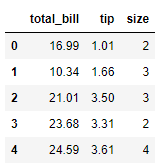
The following script imports the “tips” dataset into a Pandas dataframe and displays its header.

import pandas as pd
import numpy as np
import matplotlib.pyplot as plt
import seaborn as sns
sns.set_style("darkgrid")

tips_ds  = sns.load_dataset('tips')
tips_ds.head()

Output:

Data scaling is applied to numeric columns. In our “tips” dataset we have three numeric columns: total_bill, tip, size. The script below filters these three columns and removes the remaining columns.

tips_ds_numeric = tips_ds.filter(["total_bill", "tip", "size"], axis = 1)
tips_ds_numeric.head()

Output:

You can see from the above output that our dataset now contains just three columns. Notice the scale of data for the total_bill column is very different from the tip and size columns.

Let’s plot some statistical values for the columns in our dataset using the describe() method.

tips_ds_numeric.describe()

Output:

The above output confirms our three columns are not scaled. The mean, minimum and maximum values, and even the standard deviation values for all three columns are very different.

This unscaled dataset is not suitable for processing by some statistical algorithms. We need to scale this data so that’s exactly what we’ll do in the upcoming sections where we’ll show you different types of data scaling techniques in action.

Get Our Python Developer Kit for Free

I put together a Python Developer Kit with over 100 pre-built Python scripts covering data structures, Pandas, NumPy, Seaborn, machine learning, file processing, web scraping and a whole lot more - and I want you to have it for free. Enter your email address below and I'll send a copy your way.

Standard Scaling

Several machine learning algorithms, like linear regression support vector machines (SVMs) assume all the features in a dataset are centered around 0 and have unit variances. It’s a common practice to apply standard scaling to your data before training these machine learning algorithms on your dataset.

In standard scaling, a feature is scaled by subtracting the mean from all the data points and dividing the resultant values by the standard deviation of the data.

Mathematically, this is written as:

scaled = (x-u)/s

Here, u refers to the mean value and s corresponds to the standard deviation.

To apply standard scaling with Python, you can use the StandardScaler class from the sklearn.preprocessing module. You need to call the fit_transform() method from the StandardScaler class and pass it your Pandas Dataframe containing the features you want scaled. Here’s an example using the tips_ds_numeric dataset we made earlier.

from sklearn.preprocessing import StandardScaler

ss = StandardScaler()
tips_ds_scaled = ss.fit_transform(tips_ds_numeric)

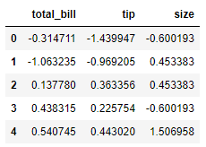
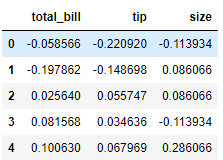
The fit_transform() method returns a NumPy array which you can convert to a Pandas Dataframe by passing the array to the Dataframe class constructor. The following script makes the conversion and prints the header for our newly scaled dataset.

tips_ds_scaled_df = pd.DataFrame(tips_ds_scaled,
                                 columns = tips_ds_numeric.columns)
tips_ds_scaled_df.head()

Output:

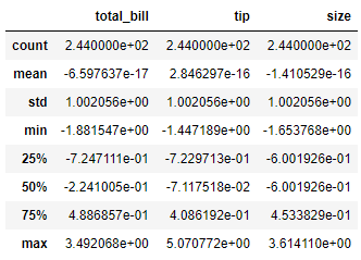
If you call the describe() function again, you’ll see that your data columns are now uniformly scaled and will have a mean centered around 0.

tips_ds_scaled_df.describe()

Output:

Min/Max Scaling

Min/Max scaling normalizes the data between 0 and 1 by subtracting the overall minimum value from each data point and dividing the result by the difference between the minimum and maximum values.

The Min/Max scaler is commonly used for data scaling when the maximum and minimum values for data points are known. For instance, you can use the min/max scaler to normalize image pixels having values between 0 and 255.

You’ll want to use the MinMaxScaler class from the sklearn.preprocessing module to perform min/max scaling. The fit_transform method of the class performs the min/max scaling on the input Pandas Dataframe, as shown below:

from sklearn.preprocessing import MinMaxScaler

mms = MinMaxScaler()
tips_ds_mms = mms.fit_transform(tips_ds_numeric)

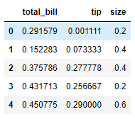
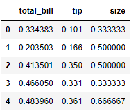
Similarly, the script below converts the NumPy array returned by the fit_transform() to a Pandas Dataframe which contains our normalized values between 0 and 1.

tips_ds_mms_df = pd.DataFrame(tips_ds_mms,
                              columns = tips_ds_numeric.columns)
tips_ds_mms_df.head()

Output:

Mean Scaling

Mean scaling is similar to min/max scaling, however in the case of mean scaling, the mean value, instead of the minimum value, is subtracted from all the data points. The result of the subtraction is divided by the range (difference between the minimum and maximum values).

Like Min/Max scaling, mean scaling is used for data scaling when the minimum and maximum values for the features to be scaled are known in advance.

The scikit-learn module by default doesn’t contain a class for the mean scaling. However, it’s very easy to implement this form of scaling in Python from scratch.

The script below finds the mean values for all three columns in our input Pandas Dataframe.

tips_means = tips_ds_numeric.mean(axis=0)
print(tips_means)

Output:

total_bill    19.785943
tip            2.998279
size           2.569672
dtype: float64

Next, the script below finds the ranges for all the features by subtracting the minimum values from the maximum values for all the columns in the input Pandas Dataframe.

min_max_range = tips_ds_numeric.max(axis=0) - tips_ds_numeric.min(axis=0)
print(min_max_range)

Output:

total_bill    47.74
tip            9.00
size           5.00
dtype: float64

The mean scaling can be performed by subtracting the data points by the mean values and dividing the result by the range, as shown in the script below:

tips_scaled_mean = (tips_ds_numeric - tips_means) / min_max_range

Finally, the script below prints the header of the Dataframe containing our newly scaled values via the mean scaling technique we just implemented without using any external scaling libraries.

tips_scaled_mean_df = pd.DataFrame(tips_scaled_mean,
                              columns = tips_ds_numeric.columns)
tips_scaled_mean_df.head()

Output:

Maximum Absolute Scaling

Maximum absolute scaling is another commonly used data scaling technique where the difference between the data points and the minimum value is divided by the maximum value. The maximum absolute scaling technique also normalizes the data between 0 and 1.

Maximum absolute scaling doesn’t shift or center the data so it’s commonly used for scaling sparse datasets.

You can use the fit_transform() method from the MaxAbsScaler class of the sklearn.preprocessing module to apply maximum absolute scaling to your dataset.

from sklearn.preprocessing import MaxAbsScaler

mas = MaxAbsScaler()
tips_ds_mas = mas.fit_transform(tips_ds_numeric)

Just like we did earlier, the script below converts the NumPy array returned by the fit_transform() method to a Pandas Dataframe and then prints the header of our scaled dataset.

tips_ds_mas_df = pd.DataFrame(tips_ds_mas,
                              columns = tips_ds_numeric.columns)
tips_ds_mas_df.head()

Output:

Median and Quantile Scaling

In median and quantile scaling, also known as robust scaling, the first step is to subtract the median value from all the data points. In the next step, the resultant values are divided by the IQR (interquartile range). The IQR is calculated by subtracting the first quartile values in your dataset from the third quartile values.

We talked about IQR values in our tutorial on handling outlier data with Python. This makes sense because median and quantile scaling is the most commonly used scaling technique for datasets with a large number of outliers.

Median and quantile scaling can be implemented via the RobustScaler class from the sklearn.preprocessing module. As with the other data scaling classes from the scikit-learn library, you need to call the fit_transform() method and pass it the input dataset, as shown in the script below:

from sklearn.preprocessing import RobustScaler

rs = RobustScaler()
tips_ds_rs = rs.fit_transform(tips_ds_numeric)

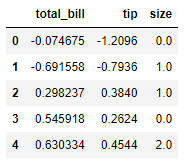
You’re probably used to this by now, but the script below converts the NumPy array containing scaled values to a Pandas DataFrame and displays the header of the Pandas dataframe.

tips_ds_rs_df = pd.DataFrame(tips_ds_rs,
                              columns = tips_ds_numeric.columns)
tips_ds_rs_df.head()

Output:

Even without using tips_ds_rs_df.describe(), you can tell just by looking at the tip and size columns that median and quantile scaling doesn’t normalize your data like many of the other scaling techniques we’ve demonstrated.

Get Our Python Developer Kit for Free

I put together a Python Developer Kit with over 100 pre-built Python scripts covering data structures, Pandas, NumPy, Seaborn, machine learning, file processing, web scraping and a whole lot more - and I want you to have it for free. Enter your email address below and I'll send a copy your way.