Techniques for Handling Outlier Data with Python

In this tutorial, we’ll learn how to remove outliers from your dataset using Python.

What are Outliers

Outliers are data values that are far outside the rest of the observations in your dataset. Depending on the context, you sometimes might hear outliers referred to as anomalies.

For example, if the age of most college going students in a dataset is between 18 and 25, an observation of 60 for the age of a student would be considered an outlier.

Outliers in some cases can be useful for detection of abnormal activities. For instance, if a person accesses her online bank account from a specific location 95% of the time and then suddenly her bank account is accessed from a geographical location far from her previous login, the new login will be treated as an outlier and can be helpful in fraud detection.

However, outliers can also occur in your dataset due to human mistakes while entering data or even a failure of a data recording device. In such cases, outliers can distort the distribution of data and convey erroneous information. If not handled, this can affect the performance of statistical algorithms like machine learning models.

In this article, we’ll show you different techniques for removing outliers from your dataset and we’ll give you examples demonstrating exactly how to implement them with Python.

Importing the Dataset

The following script imports the libraries required to execute scripts in this article, along with the dataset. The dataset comes built-in with the Seaborn library, which is stored in a Pandas dataframe using the load_dataset() method in the script below:

import pandas as pd
import numpy as np
import matplotlib.pyplot as plt
import seaborn as sns
sns.set_style("darkgrid")
plt.rcParams["figure.figsize"] = [8,6]


tips_ds  = sns.load_dataset('tips')
tips_ds.head()

The output below shows the header (first five rows) of our dataset. Our dataset contains information for bills paid at a fictional restaurant. The dataset contains values for the total amount of the bill, the tip, the day and time of the bill, and the gender of the person who paid the bill.

Output:

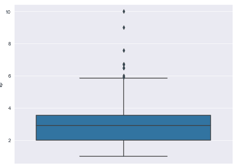
One of the fastest ways to get a look at the outliers in your dataset is via a box plot. The following script makes a box plot for the “tips” column of our dataset.

sns.boxplot( y='tip', data=tips_ds)

Output:

The lower border of the blue box in the figure above shows the first quartile - 25% of the tip values in our dataset fall below this range. The line in the middle of the blue box shows the 2nd quartile or median. 50% of the tip values occur below this range. The upper border of the blue box in the figure below shows the third quartile. 75% of the tips values in our dataset occur below this range.

The difference between the 3rd and 1st quartile is called the interquartile-range (IQR).

The horizontal line at the bottom of the box plot is called the lower limit and is calculated here as:

lower limit = Quartile One (q1) -  IQR x 1.5

The horizontal line at the top is called the upper limit and is calculated as:

upper limit = Quartile three (q3) +  IQR x 1.5

The points below or above the lower and upper limits can be considered outliers. In the figure below, you can see several black dots above the upper limit. We’re going to treat these as outlier values.

So how do you remove these values from your dataset? Let’s take a look.

Get Our Python Developer Kit for Free

I put together a Python Developer Kit with over 100 pre-built Python scripts covering data structures, Pandas, NumPy, Seaborn, machine learning, file processing, web scraping and a whole lot more - and I want you to have it for free. Enter your email address below and I'll send a copy your way.

Trimming Outliers using IQR Ranges

One of the ways to remove outliers from your dataset is by removing all the values above or below the upper and lower limits calculated with IQR ranges.

Outlier trimming via the IQR range does not distort the default data distribution and therefore can be used when the dataset is not follow a normal (Gaussian) distribution.

Let’s find the quartile one (q1) and quartile three (q3) values for the tips column of our dataset. These values will be used to find the IQR range.

q3 = tips_ds["tip"].quantile(0.75)  
q1 = tips_ds["tip"].quantile(0.25)
print(q3)
print(q1)

Output:

3.5625
2.0

The IQR range can be calculated by simply subtracting the q1 value from q3. The following script finds and prints the IQR value.

IQR = q3 - q1
print(IQR)

Output:

1.5625

The lower limit is calculated by multiplying the IQR value by 1.5 and then subtracting the resulting value from q1. The following script does that.

lower_limit = q1 - (IQR * 1.5)
print(lower_limit)

Output:

-0.34375

Similarly, the script below calculates and prints the upper limit.

upper_limit = q3 + (IQR * 1.5)
print(upper_limit)

Output:

5.90625

Once you have the upper and lower limits for your outliers, you can filter the data from your Pandas dataframe where the tip column contains values between your upper and lower limits. The following script returns rows that contain outlier values.

tips_outliers = np.where(tips_ds["tip"] > upper_limit, True,
                np.where(tips_ds["tip"] < lower_limit, True, False))

The script below then removes these outlier rows from our original dataset.

tips_without_outliers = tips_ds.loc[~(tips_outliers)]

Our next script prints the shape of our original and our new filtered dataset.

print(tips_ds.shape)
print(tips_without_outliers.shape)

Output:

(244, 7)
(235, 7)

The output shows that 9 records were classified as outliers and have been removed from our original dataset.

Finally, we can create a new box plot to see our new data distribution.

sns.boxplot( y='tip', data=tips_without_outliers)

Output:

The output below shows you now only have a single outlier in your new distribution. Do not worry. This record wasn’t considered an outlier in our original distribution and only shows as an outlier now because of the new dataset means we have new IQR calculations. It’s perfectly fine to keep it since it wasn’t an outlier in our original set.

Capping Outliers using IQR Ranges

Trimming outliers altogether may result in the removal of a large number of records from your dataset which isn’t desirable in some cases since columns other than the ones containing the outlier values may contain useful information.

In such cases, you can use outlier capping to replace the outlier values with a maximum or minimum capped values. Be warned, this manipulates your data, but here’s how you do it.

You can replace outlier values by the upper and lower limit calculated using the IQR range in the last section. Look at the following script for reference.

tips_ds["tip_capped"] = np.where(tips_ds["tip"]> upper_limit, upper_limit,
                        np.where(tips_ds["tip"]< lower_limit, lower_limit,
                          tips_ds["tip"]))

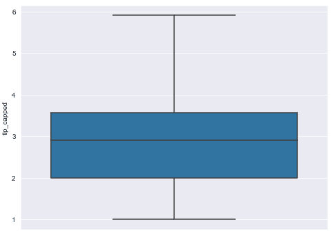
Now if you plot your dataset, you will see that all the outliers are removed from the original distribution.

sns.boxplot( y="tip_capped", data=tips_ds)

Output:

Get Our Python Developer Kit for Free

I put together a Python Developer Kit with over 100 pre-built Python scripts covering data structures, Pandas, NumPy, Seaborn, machine learning, file processing, web scraping and a whole lot more - and I want you to have it for free. Enter your email address below and I'll send a copy your way.

Capping Outliers using Fixed Quantiles

You can also used fixed quantile values to replace outlier values with capped values.

For instance, you may want to consider values as outliers if they are less than or more than the values for 97% of all the records in your dataset. In such cases you can use the quantile() method of the Pandas dataframe and pass it thresholds for lower and upper limits.

For instance, a threshold value of 0.03 for the quantile() method will find the values that are less than 97% of all the records in the dataset. Where as a threshold value of 97% returns values that are greater than 97% of the records. The following script finds the upper and lower limits for outliers using these fixed quantiles.

lower_limit = tips_ds["tip"].quantile(0.03)  
upper_limit = tips_ds["tip"].quantile(0.97)

print(lower_limit)
print(upper_limit)

Output:

1.25
5.976799999999998

You can then replace the outlier values with the upper and lower limits using the following script.

tips_ds["tip_capped"] = np.where(tips_ds["tip"]> upper_limit, upper_limit,
                        np.where(tips_ds["tip"]< lower_limit, lower_limit,
                        tips_ds["tip"]))

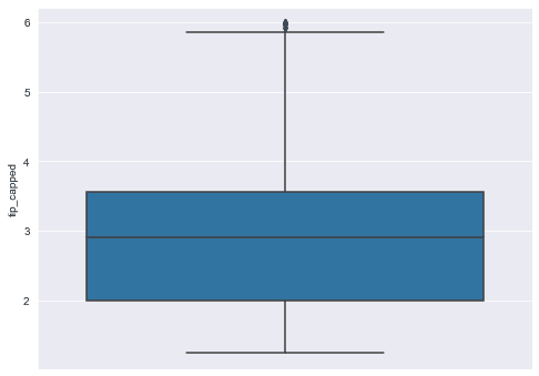
Here is the box plot for the new distribution achieved by capping outliers using fixed quantile values.

sns.boxplot( y="tip_capped", data=tips_ds)

Output:

It’s worth mentioning that 97% is chosen arbitrarily here and since we did a lower and upper cap, we’re essentially retaining the central 94% of our data. Recall that for a normal distribution 68% of your data falls within 1 standard deviation, 95% falls within 2 standard deviations and 99.7% falls within 3 standard deviations. We’ll talk more about standard deviations and how they can be used for robust outlier handling of a normal distribution in this next section.

Capping Outliers using Mean and Standard Deviations

Another way of capping outliers is by using the mean and standard deviation values. This approach is very useful when your data is normally distributed (Gaussian) around a central mean.

In this approach, the lower bound value for the outlier is calculated by subtracting three standard deviations from the mean value. Similarly, the upper bound is calculated by adding three standard deviation value to the mean value. Look at the script below:

lower_limit = tips_ds["tip"].mean() - (3 * tips_ds["tip"].std())
upper_limit = tips_ds["tip"].mean() + (3 * tips_ds["tip"].std())

print(lower_limit)
print(upper_limit)

Output:

-1.152635878478958
7.149193255528139

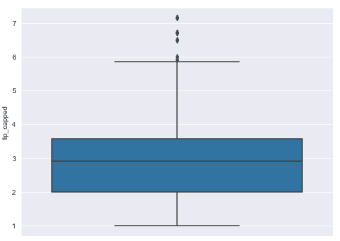
The rest of the process is follows the same steps we’ve seen before. The lower bound and upper bound values are used to replace the outlier values, as shown in the script below:

tips_ds["tip_capped"] = np.where(tips_ds["tip"]> upper_limit, upper_limit,
                        np.where(tips_ds["tip"]< lower_limit, lower_limit,
                        tips_ds["tip"]))

sns.boxplot( y="tip_capped", data=tips_ds)

Output:

Trimming Outliers using Mean and Standard Deviations

If you’d rather not replace the values outside 3 standard deviations, you can delete them using this script, just like we did in our first section. I find this method to be the most valuable so I put the entire code here to make it easier for you to copy and paste.

import pandas as pd
import numpy as np
import matplotlib.pyplot as plt
import seaborn as sns
sns.set_style("darkgrid")
plt.rcParams["figure.figsize"] = [8,6]


tips_ds  = sns.load_dataset('tips')
lower_limit = tips_ds["tip"].mean() - (3 * tips_ds["tip"].std())
upper_limit = tips_ds["tip"].mean() + (3 * tips_ds["tip"].std())

tips_outliers = np.where(tips_ds["tip"]> upper_limit, True,
                np.where(tips_ds["tip"]< lower_limit, True, False))

tips_without_outliers = tips_ds.loc[~(tips_outliers)]

sns.boxplot( y='tip', data=tips_without_outliers)

Capping Outliers using Custom Values

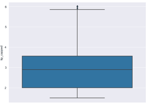
Finally, you can use your own custom values based on your knowledge of expected values in your dataset to replace outliers. For instance, if you think that the tip values greater than 6 and less than 1.5, are outliers, you can replace these values with a custom value. Here’s a script for your reference.

lower_limit = 1.5
upper_limit = 6.0

tips_ds["tip_capped"] = np.where(tips_ds["tip"]> upper_limit, upper_limit,
                        np.where(tips_ds["tip"]< lower_limit, lower_limit,
                        tips_ds["tip"]))

sns.boxplot( y="tip_capped", data=tips_ds)

Output:

Whichever method you decide to use for handling outlier data depends on your use case. This tutorial deletes or replaces your outlier data and stores your new data in a Pandas dataframe. Whatever you do after that is up to you! For suggestions on neat ways to manipulate and process your data, subscribe using the form below.

Get Our Python Developer Kit for Free

I put together a Python Developer Kit with over 100 pre-built Python scripts covering data structures, Pandas, NumPy, Seaborn, machine learning, file processing, web scraping and a whole lot more - and I want you to have it for free. Enter your email address below and I'll send a copy your way.