In this tutorial, we’re going show you how to implement logistic regression for binary classification in Python from scratch - without using any machine learning library.
Logistic regression is a machine learning algorithm commonly used for binary classification tasks. A binary classification task involves classifying input data into one of the two predefined classes.
Many advanced machine learning libraries, like Sklearn, and TensorFlow, implement logistic regression algorithms in a few lines of code. However, it can be valuable to understand what’s happening inside the logistic regression algorithm if you are a new data scientist or even an advanced machine learning researcher. And the best way to understand what’s happening inside is by implementing the algorithm from scratch. That’s precisely what we’re going to do today.
Creating a Dummy Dataset
Machine learning algorithms, such as logistic regression, are trained on data. Once trained on the training dataset, an algorithm can make predictions on the unseen dataset.
We’re going to create a dummy dataset with two features for demonstration purposes in this tutorial. The output for each record will be 0 or 1 since our intention is to solve a binary classification problem.
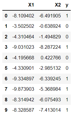
The following script creates the dummy dataset and plots the first ten records. The dataset contains 500 instances in total.
In the output, you can see two dataset features, X1 and X2, and the target label y, which contains 1 or 0. We’re going to use sklearn to make this sample dataset and split it into test and training sets, but we’re not going to use it to implement our logistic regression model.
from sklearn.datasets import make_blobs

X, y = make_blobs(n_samples=500, centers=2, n_features=2)

import pandas as pd

dataset = pd.DataFrame(X, columns = ["X1", "X2"])
dataset["y"] = y
dataset.head(10)
Output:
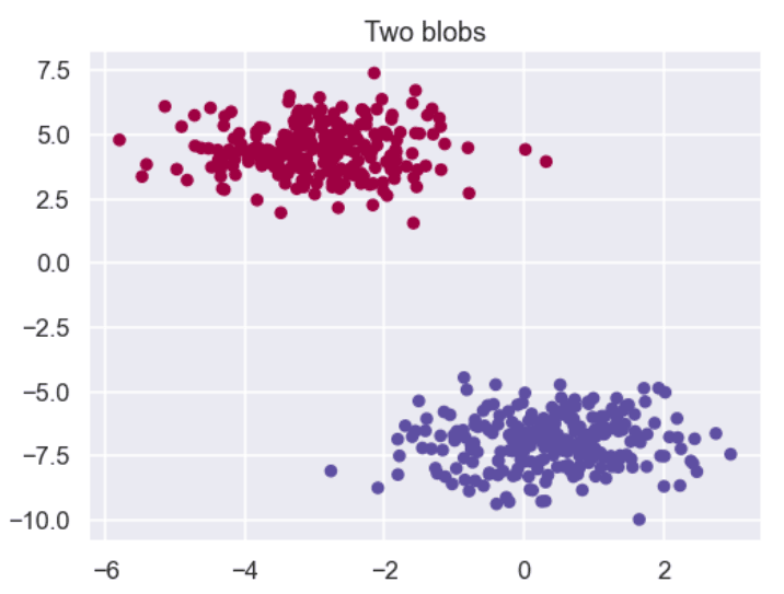
Let’s plot our dataset on a 2-D axis. The output of the below script shows that our dataset is linearly separable, which means that a straight line can separate the two classes of target labels in our dataset. Logistic regression is a perfect choice if a straight line can separate your dataset since Logistic regression essentially finds that straight line.
from matplotlib import pyplot
import seaborn as sns
sns.set_style("darkgrid")
sns.set_context("talk")

pyplot.figure(figsize=(8, 6))
pyplot.title("Two blobs")
pyplot.scatter(X[:, 0], X[:, 1], marker="o", c=y, s=50, cmap ="Spectral")
Output:
Lets’s print the shape of our dataset:
print(X.shape)
print(y.shape)
Output:
(500, 2)
(500,)
Our feature set consists of 500 rows and 2 columns; however, the target labels set y is a one-dimensional vector. We need to convert it into a row vector that corresponds to rows in the feature set, as shown in the following script:
y = y.reshape(y.shape[0],1)
print(y.shape)
Output:
(500, 1)Both target labels set now consists of 500 rows and 1 column.
Finally, we’ll divide our dataset into 80% training and 20% test sets. We will train the logistic regression algorithm we’re building from scratch on the 80% training set and evaluate the trained model by making predictions on the 20% test set.
from sklearn.model_selection import train_test_split
X_train, X_test, y_train, y_test = train_test_split(X, y, test_size=0.2, random_state=25)
The logistic regression algorithm consists of two steps: a forward pass and a backward pass.
Forward Pass
In forward pass, you make predictions on the training set. For the logistic regression algorithm, the formula for the forward pass is:
A = Sigmoid (XW + B)
I know you must be wondering where these XW and B variables come from. Let me explain that.
As I mentioned earlier, the logistic regression algorithm finds a straight line that separates your dataset.
The equation of a straight line is:
XW + b
where X is the input features of your dataset. W stands for the weights in the above equation. The term XW is the dot product of X and W. The term B represents the intercept and is used to calculate the default prediction value in case all the weights are zero. Perhaps you recall seeing the formula for a straight line as y = mx + b. It’s the same concept for the forward pass.
Since X remains constant, the only way to control the slope of the straight line is by updating the weights and bias values.
The equation XW + b outputs a real value depending upon the weights and bias values. Our output target labels are 0 and 1. One approach to force the output of the equation XW + B between 0 and 1 is by using the sigmoid function.
The sigmoid function outputs a value between 0.5 and 1 if the input to the function is positive. Larger positive inputs result in an output close to 1. For the cases where the input is negative, the sigmoid function outputs a value between 0 and 0.5. Larger negative inputs result in values closer to 0.
The output of the sigmoid function can be treated as probability values. In logistic regression, we convert predicted values >= 0.5 to 1, and the predicted values from 0 to < 5.
The following script defines the sigmoid function.
def sigmoid(x):
    s = 1/(1+np.exp(-x))
    return s
Note: np is going to be defined later with the line import numpy as np.
The script below defines the function for the logistic regression predictions.
def make_predictions(X, W, b):
    Z = np.dot(X,W) + b
    A = sigmoid (Z)
    return A
We need a loss function to find the best weights and bias values. The loss function shows how good or bad our logistic regression model performs.
The binary cross-entropy function is one of the most commonly used loss functions for logistic regression. However, you can use the mean squared error loss function as well.
The following script contains a Python implementation of the binary cross-entropy function.
def calculate_loss(Y,Y_hat):
    loss = np.mean(-((Y * np.log(Y_hat)) + ((1-Y)*np.log(1-Y_hat))))

    return loss
The core task in any machine learning problem is to minimize the loss function, which entails finding weights and bias values that return minimum values for the loss function. The backpropagation step performs this task.
Backpropagation
In backpropagation you start with random initial values for weights and biases, as shown in the following script:
import numpy as np

W = np.random.rand(X.shape[1], y.shape[1])
print(W)

b = 0
print(b)
Output:
[[0.41028886]
 [0.45758508]]
0
The dimension of the matrix W is [2,1] since we have 2 features in the dataset, and we want to calculate one value in the output.
Let’s first see what prediction accuracy we get on the test set with the randomly initialized weights.
from sklearn.metrics import classification_report
from sklearn.metrics import accuracy_score


predictions = make_predictions(X_test, W, b)
predictions[:10]

y_pred = [1 if pred > 0.5 else 0 for pred in predictions]


print(classification_report(y_test, y_pred))
print(accuracy_score(y_test, y_pred))
Output:
precision    recall  f1-score   support

0       0.00      0.00      0.00      50.0
1       0.00      0.00      0.00      50.0

accuracy                           0.00     100.0
macro avg       0.00      0.00      0.00     100.0
weighted avg       0.00      0.00      0.00     100.0

0.0
The above output shows that we do not get a single prediction right with random weights.
We need to find the weights and bias values that give us the best accuracy, or in other words, minimize the loss.
The gradient descent algorithm is the most commonly used method for minimizing the loss of a function.
In gradient descent for a loss function, you find the function’s gradient (derivative) with respect to weights and biases at a particular instance; then, you move the weights and biases in a direction that reduces the loss. You keep repeating the process until you find the weights and bias values resulting in the minimum loss.
The following script defines the method that finds the gradient of the binary cross entropy function with respect to weights and bias values. Refer to this excellent article to see the mathematical details of finding the gradient (derivative) of the binary cross entropy function.
def find_gradient(X, Y, W, b, A):

    dw = np.dot(X.T, (A-Y))/X_train.shape[0]
    db = np.sum(A-Y)/X_train.shape[0]

    return dw, db
Finally, to move the weights and biases in the direction that minimizes the loss function, you can subtract the gradients from the original weights and bias values, as shown in the following script. Here lr refers to the learning rate, which defines the magnitude of updates in weights and bias values. When fully implemented, it’s going to look something like this:
dw, db = find_gradient(X, y, W, b, A)

W = W - lr * dw
b = b - lr * b
Train the Logistic Regression Model
We are now ready to train our logistic regression model. The following script defines the train_model() method that performs the forward pass and backpropagation.
The epochs here refers to the number of iterations for training the logistic regression algorithm on your training set.
def train_model(X, y, W, b, epochs, lr):

    lr = lr

    loss_vals = []

    for i in range(epochs):

        ## Forward Pass

        A = make_predictions(X, W, b)
        loss = calculate_loss(y, A)

        if (i%100) == 0:
            print("loss at iteration" , i, loss)
        loss_vals.append(loss)

        ## Backpropagation

        dw, db = find_gradient(X, y, W, b, A)

        W = W - lr * dw
        b = b - lr * b

    return W, b, loss_vals
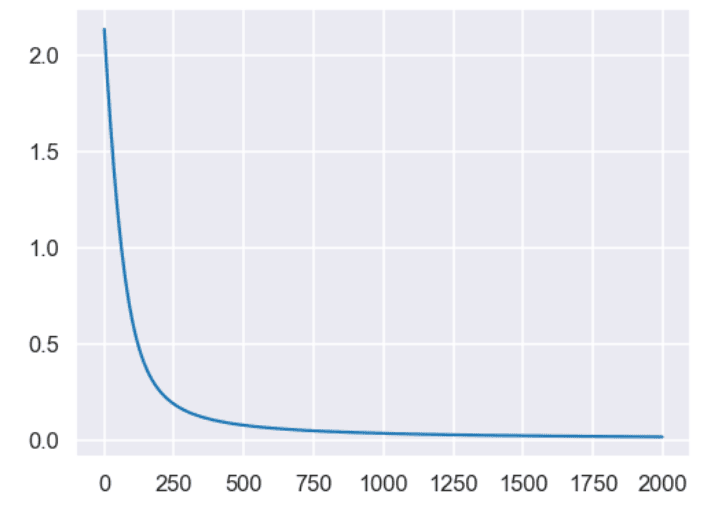
Let’s train our logistic regression model for 2000 epochs. The loss is plotted every 100 iterations.
lr = 0.001
epochs = 2000

W, b, loss_vals = train_model(X_train, y_train, W, b, epochs, lr)
Output:
loss at iteration 0 2.1373284933253824
loss at iteration 100 0.626349853224586
loss at iteration 200 0.2547537983189216
loss at iteration 300 0.14822885404706362
loss at iteration 400 0.10310681466649604
loss at iteration 500 0.07888820974996111
loss at iteration 600 0.06392129287720455
loss at iteration 700 0.05379041812592839
loss at iteration 800 0.04648718911517035
loss at iteration 900 0.04097486811407867
loss at iteration 1000 0.03666656150679531
loss at iteration 1100 0.03320592433777645
loss at iteration 1200 0.030364381730720334
loss at iteration 1300 0.02798869615570923
loss at iteration 1400 0.02597234256385208
loss at iteration 1500 0.024238990486122377
loss at iteration 1600 0.02273252217301158
loss at iteration 1700 0.021410760402838794
loss at iteration 1800 0.020241393280779788
loss at iteration 1900 0.01919924866278047
You can see from the above output that the loss is constantly decreasing. Let’s plot the loss against the number of epochs.
pyplot.figure(figsize=(8, 6))

x = [loss_vals.index(i) for i in loss_vals]
pyplot.plot(x, loss_vals)
pyplot.show()
Output:
The following script plots the weights and bias values after training:
print(W)
print(b)
Output:
[[ 0.58949794]
 [-0.59200312]]
0.0
Making Predictions and Evaluating The Model
Loss values are indicators of how well your model is performing. However, you want your model to do well in the production environment, so you must evaluate how well your model is performing on a test set.
The following script makes predictions on our test set using the new weights and bias values learned via backpropagation. The first 10 target labels are printed in the output:
predictions = make_predictions(X_test, W, b)
predictions[:10]
Output:
array([[0.0207298 ],
       [0.98152343],
       [0.01458247],
       [0.00256471],
       [0.01455384],
       [0.99535977],
       [0.04171803],
       [0.98855056],
       [0.00748652],
       [0.03165435]])
The above values are the output of the sigmoid function. To convert it into binary values, you can use the probability rule where all values greater than 0.5 are converted to 1, and the values less than 0.5 are converted to 0.
y_pred = [1 if pred > 0.5 else 0 for pred in predictions]
y_pred[:10]
Output:
[0, 1, 0, 0, 0, 1, 0, 1, 0, 0]Finally, you can calculate recall, precision, F1 value, and accuracy of your model on the test set via the following script:
from sklearn.metrics import classification_report
from sklearn.metrics import accuracy_score

print(classification_report(y_test, y_pred))
print(accuracy_score(y_test, y_pred))
Output:
precision    recall  f1-score   support

0       1.00      1.00      1.00        50
1       1.00      1.00      1.00        50

accuracy                           1.00       100
macro avg       1.00      1.00      1.00       100
weighted avg       1.00      1.00      1.00       100

1.0
The output shows that our model’s accuracy is 100%, as it correctly predicts the target labels for all the instances in the test set.
If you’re ready to learn more about machine learning and how you can use Python to perform all kinds of machine learning tasks, enter your email address in the form below!


